Note
Go to the end to download the full example code.
EEG speech envelope TRF
A TRF analysis on data that comes as arrays. Analyze continuous speech data from the mTRF dataset [1]. Use the boosting algorithm for estimating temporal response functions (TRFs) to the acoustic envelope.
# Author: Christian Brodbeck <christianbrodbeck@nyu.edu>
# sphinx_gallery_thumbnail_number = 4
import os
from scipy.io import loadmat
import mne
from eelbrain import *
# Load the mTRF speech dataset and convert data to NDVars
root = mne.datasets.mtrf.data_path()
speech_path = os.path.join(root, 'speech_data.mat')
mdata = loadmat(speech_path)
# Time axis
tstep = 1. / mdata['Fs'][0, 0]
n_times = mdata['envelope'].shape[0]
time = UTS(0, tstep, n_times)
# Load the EEG sensor coordinates (drop fiducials coordinates, which are stored
# after sensor 128)
sensor = Sensor.from_montage('biosemi128')[:128]
# Frequency dimension for the spectrogram
band = Scalar('frequency', range(16))
# Create variables
envelope = NDVar(mdata['envelope'][:, 0], (time,), name='envelope')
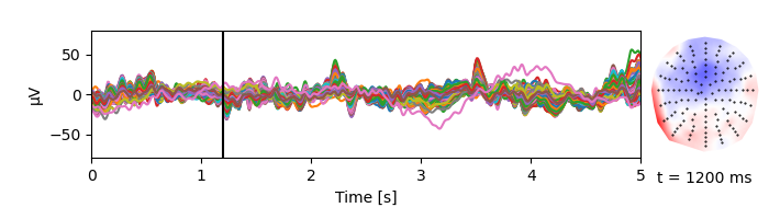
eeg = NDVar(mdata['EEG'], (time, sensor), name='EEG', info={'unit': 'µV'})
spectrogram = NDVar(mdata['spectrogram'], (time, band), name='spectrogram')
# Exclude a bad channel
eeg = eeg[sensor.index(exclude='A13')]
Data
Plot the spectrogram of the speech stimulus:
plot.Array(spectrogram, xlim=5, w=6, h=2)
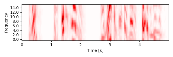
<Array: spectrogram>
Plot the envelope used as stimulus representation for TRFs:
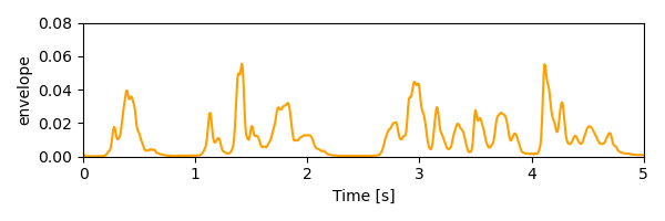
<UTS: envelope>
Plot the corresponding EEG data:
p = plot.TopoButterfly(eeg, xlim=5, w=7, h=2)
p.set_time(1.200)
TRF estimation
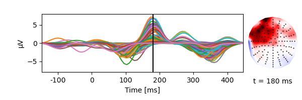
TRF for the envelope using boosting:
TRF from -100 to 400 ms
Basis of 100 ms Hamming windows
Use 4 partitionings of the data for cross-validation based early stopping
res = boosting(eeg, envelope, -0.100, 0.400, basis=0.100, partitions=4)
p = plot.TopoButterfly(res.h_scaled, w=6, h=2)
p.set_time(.180)
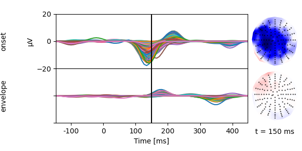
Multiple predictors
Multiple predictors additively explain the signal:
# Derive acoustic onsets from the envelope
onset = envelope.diff('time', name='onset').clip(0)
onset *= envelope.max() / onset.max()
plot.UTS([[envelope, onset]], xlim=5, w=6, h=2)
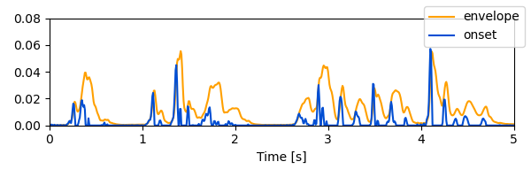
<UTS: envelope, onset>
res_onset = boosting(eeg, [onset, envelope], -0.100, 0.400, basis=0.100, partitions=4)
p = plot.TopoButterfly(res_onset.h_scaled, w=6, h=3)
p.set_time(.150)
Compare models
Compare model quality through the correlation between measured and predicted responses:
plot.Topomap([res.r, res_onset.r], w=4, h=2, columns=2, axtitle=['envelope', 'envelope + onset'])
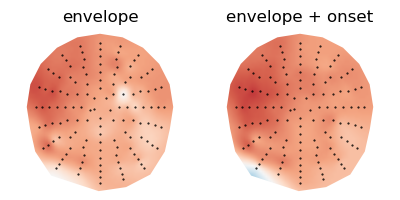
<Topomap: Correlation>
References
Total running time of the script: (0 minutes 29.935 seconds)