ANCOVA

Analysis of covariance for univariate data.

Example 1

Based on [1], Exercises (page 8).

# Author: Christian Brodbeck <christianbrodbeck@nyu.edu>
from eelbrain import *

y = Var([2, 3, 3, 4,
         3, 4, 5, 6,
         1, 2, 1, 2,
         1, 1, 2, 2,
         2, 2, 2, 2,
         1, 1, 2, 3], name="Growth Rate")

genotype = Factor(range(6), repeat=4, name="Genotype")

hours = Var([8, 12, 16, 24], tile=6, name="Hours")

Show the model

print(hours * genotype)
intercept   Hours   Genotype                 Hours x Genotype
-----------------------------------------------------------------------------
1           8       1    0    0    0    0    8      0      0      0      0
1           12      1    0    0    0    0    12     0      0      0      0
1           16      1    0    0    0    0    16     0      0      0      0
1           24      1    0    0    0    0    24     0      0      0      0
1           8       0    1    0    0    0    0      8      0      0      0
1           12      0    1    0    0    0    0      12     0      0      0
1           16      0    1    0    0    0    0      16     0      0      0
1           24      0    1    0    0    0    0      24     0      0      0
1           8       0    0    1    0    0    0      0      8      0      0
1           12      0    0    1    0    0    0      0      12     0      0
1           16      0    0    1    0    0    0      0      16     0      0
1           24      0    0    1    0    0    0      0      24     0      0
1           8       0    0    0    1    0    0      0      0      8      0
1           12      0    0    0    1    0    0      0      0      12     0
1           16      0    0    0    1    0    0      0      0      16     0
1           24      0    0    0    1    0    0      0      0      24     0
1           8       0    0    0    0    1    0      0      0      0      8
1           12      0    0    0    0    1    0      0      0      0      12
1           16      0    0    0    0    1    0      0      0      0      16
1           24      0    0    0    0    1    0      0      0      0      24
1           8       0    0    0    0    0    0      0      0      0      0
1           12      0    0    0    0    0    0      0      0      0      0
1           16      0    0    0    0    0    0      0      0      0      0
1           24      0    0    0    0    0    0      0      0      0      0

Estimate the ANCOVA:
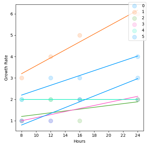
test.ANOVA(y, hours * genotype)
SS df MS F p
Hours 7.06 1 7.06 54.90*** < .001
Genotype 27.88 5 5.58 43.36*** < .001
Hours x Genotype 3.15 5 0.63 4.90* .011
Residuals 1.54 12 0.13
Total 39.62 23


Plot the slopes:

ANCOVA

Example 2

Based on [2] (p. 118-20)

y = Var([16,  7, 11,  9, 10, 11,  8,  8,
         16, 10, 13, 10, 10, 14, 11, 12,
         24, 29, 10, 22, 25, 28, 22, 24])

cov = Var([9, 5, 6, 4, 6, 8, 3, 5,
           8, 5, 6, 5, 3, 6, 4, 6,
           5, 8, 3, 4, 6, 9, 4, 5], name='cov')

a = Factor([1, 2, 3], repeat=8, name='A')

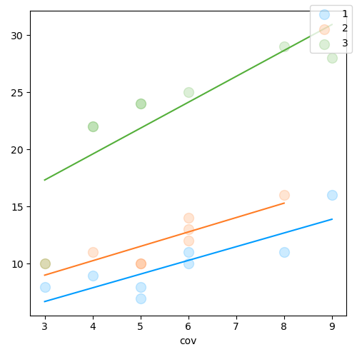
Full model, with interaction

plot.Regression(y, cov, a)
test.ANOVA(y, cov * a)
ANCOVA
SS df MS F p
cov 199.54 1 199.54 32.93*** < .001
A 807.82 2 403.91 66.66*** < .001
cov x A 19.39 2 9.70 1.60 .229
Residuals 109.07 18 6.06
Total 1112.00 23


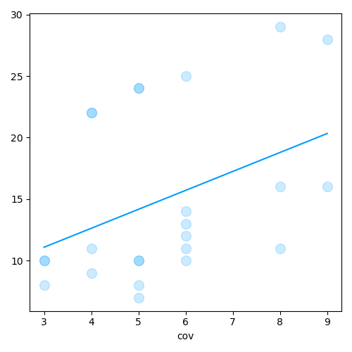
Drop interaction term

plot.Regression(y, cov)
test.ANOVA(y, a + cov)
ANCOVA
SS df MS F p
A 807.82 2 403.91 62.88*** < .001
cov 199.54 1 199.54 31.07*** < .001
Residuals 128.46 20 6.42
Total 1112.00 23


ANCOVA with multiple covariates

Based on [3], p. 139.

# Load data form a text file
ds = load.txt.tsv('Fox_Prestige_data.txt', delimiter=' ', skipinitialspace=True)
ds.head()
# id education income women prestige census type
0 GOV.ADMINISTRATORS 13.11 12351 11.16 68.8 1113 prof
1 GENERAL.MANAGERS 12.26 25879 4.02 69.1 1130 prof
2 ACCOUNTANTS 12.77 9271 15.7 63.4 1171 prof
3 PURCHASING.OFFICERS 11.42 8865 9.11 56.8 1175 prof
4 CHEMISTS 14.62 8403 11.68 73.5 2111 prof
5 PHYSICISTS 15.64 11030 5.13 77.6 2113 prof
6 BIOLOGISTS 15.09 8258 25.65 72.6 2133 prof
7 ARCHITECTS 15.44 14163 2.69 78.1 2141 prof
8 CIVIL.ENGINEERS 14.52 11377 1.03 73.1 2143 prof
9 MINING.ENGINEERS 14.64 11023 0.94 68.8 2153 prof


# Variable summary
ds.summary()
Key Type Values
id Factor GOV.ADMINISTRATORS, GENERAL.MANAGERS, ACCOUNTANTS... (102 cells)
education Var 6.38 - 15.97
income Var 611 - 25879
women Var 0 - 97.51
prestige Var 14.8 - 87.2
census Var 1113 - 9517
type Factor prof:31, bc:44, wc:23, NA:4
Fox_Prestige_data.txt: 102 cases


# Exclude cases with missing type
ds2 = ds[ds['type'] != 'NA']

# ANOVA
test.ANOVA('prestige', '(income + education) * type', data=ds2)
SS df MS F p
income 1131.90 1 1131.90 28.35*** < .001
education 1067.98 1 1067.98 26.75*** < .001
type 591.16 2 295.58 7.40** .001
income x type 951.77 2 475.89 11.92*** < .001
education x type 238.40 2 119.20 2.99 .056
Residuals 3552.86 89 39.92
Total 28346.88 97


References

Gallery generated by Sphinx-Gallery