Creating NDVars

Shows how to initialize an NDVar with the structure of EEG data from (randomly generate) data arrays. The data is intended for illustrating EEG analysis techniques and meant to vaguely resemble data from an N400 experiment, but it is not meant to be a physiologically realistic simulation.

# sphinx_gallery_thumbnail_number = 3
import numpy as np
import scipy.spatial
from eelbrain import *

NDVars from arrays

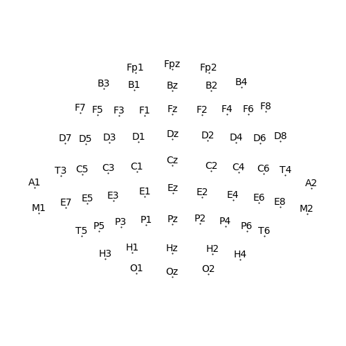
An NDVar combines an n-dimensional numpy.ndarray with Dimension objects that describe what the different data axes mean, and provide meta information that is used, for example, for plotting. Here we start by create a Sensor dimension from a built-in EEG montage (a montage pairs sensor names with spatial locations on the head surface):

sensor = Sensor.from_montage('standard_alphabetic')
p = plot.SensorMap(sensor)

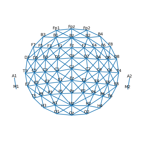
The dimension also contains information about the adjacency of its elements (i.e., specifying which elements are adjacent), which is used, for example, for cluster-based analysis. This information is imported automatically from mne when available; otherwise it can be defined manually when creating the sensor object, or based on pairwise sensor distance, as here:

sensor.set_adjacency(connect_dist=1.66)
p = plot.SensorMap(sensor, adjacency=True)

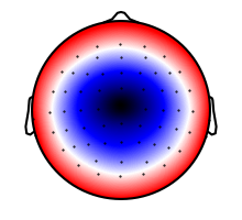
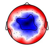
Using information from the Sensor description about sensor coordinates, we can now generate an N400-like topography. After associating the data array with the Sensor description by creating an NDVar, the topography can be plotted without any further information:

i_cz = sensor.names.index('Cz')
cz_loc = sensor.locations[i_cz]
dists = scipy.spatial.distance.cdist([cz_loc], sensor.locations)[0]
dists /= dists.max()
topo = -0.7 + dists
n400_topo = NDVar(topo, sensor)
p = plot.Topomap(n400_topo, clip='circle')

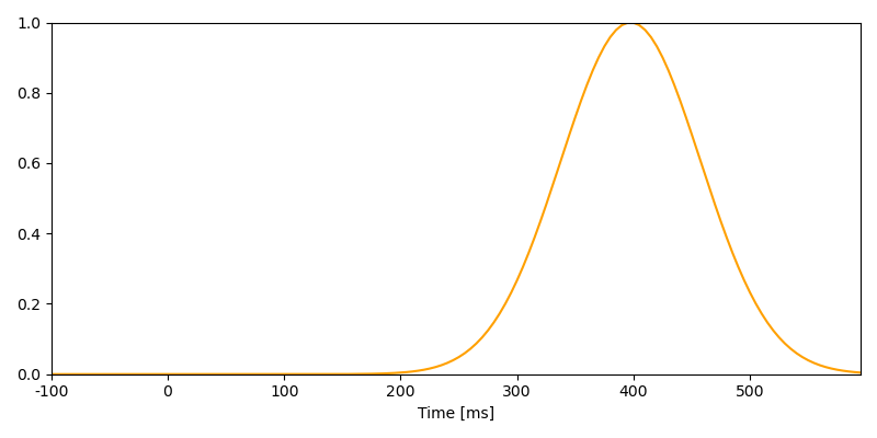
A time axis is specified using a UTS (“uniform time series”) object. As with the topography, the UTS object allows the NDVar to automatically format the time axis of a figure. Here we create a simple time series based on a Gaussian:

window_data = scipy.signal.windows.gaussian(200, 12)[:140]
time = UTS(tmin=-0.100, tstep=0.005, nsamples=140)
n400_timecourse = NDVar(window_data, time)
p = plot.UTS(n400_timecourse)

Combining NDVars

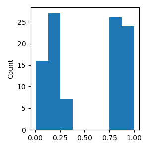
More complex NDVars can often be created by combining simpler NDVars. As example data, we generate random values for an independent variable (consistent with simulating an N400 response, we call it “cloze probability”)

rng = np.random.RandomState(0)
n_trials = 100
cloze = np.concatenate([
    rng.uniform(0, 0.3, n_trials // 2),
    rng.uniform(0.8, 1.0, n_trials // 2),
])
rng.shuffle(cloze)
p = plot.Histogram(cloze)

Stacking NDVars

A simple way of combining multiple NDVars is stacking them. Here we generate a separate topography for each cloze value, add some random noise, and then stack the resulting NDVars using combine(). The resulting stacked NDVar has a Case dimension reflecting the different cases (or trials):

ndvars = []
for cloze_i in cloze:
    topo_i = NDVar(topo * cloze_i + rng.normal(0, .5, len(topo)), sensor)
    ndvars.append(topo_i)
topographies = combine(ndvars)
topographies

<NDVar: 100 case, 65 sensor>

The resulting NDvar can directly be used for a statistical test:

result = testnd.TTestOneSample(topographies)
p = plot.Topomap(result, clip='circle')
result

Permutation test:   0%|          | 0/10000 [00:00<?, ? permutations/s]
Permutation test:  29%|██▊       | 2864/10000 [00:00<00:00, 27535.03 permutations/s]
Permutation test:  62%|██████▏   | 6168/10000 [00:00<00:00, 30719.78 permutations/s]
Permutation test:  95%|█████████▍| 9456/10000 [00:00<00:00, 31691.35 permutations/s]
Permutation test: 100%|██████████| 10000/10000 [00:00<00:00, 31198.77 permutations/s]

<TTestOneSample '<NDVar>', samples=10000, p < .001>

Casting NDVars

Multi-dimensional NDVars can also be created through multiplication of NDVars with different dimensions. Here, we put all the dimensions together to simulate the EEG signal. On the first line, turn cloze into Var to make clear that cloze represents a Case dimension, i.e. different trials:

signal = Var(1 - cloze) * n400_timecourse * n400_topo

# Add noise
noise = powerlaw_noise(signal, 1)
noise = noise.smooth('sensor', 0.02, 'gaussian')
signal += noise

# Apply the average mastoids reference
signal -= signal.mean(sensor=['M1', 'M2'])

# Store EEG data in a Dataset with trial information
ds = Dataset({
    'eeg': signal,
    'cloze': Var(cloze),
    'predictability': Factor(cloze > 0.5, labels={True: 'high', False: 'low'}),
})

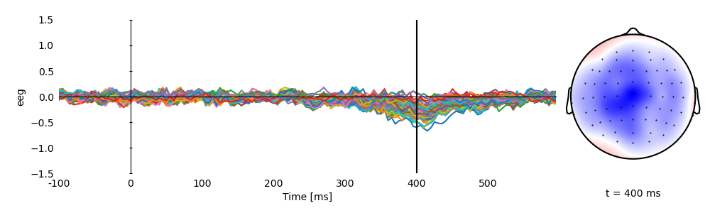
Plot the average simulated response

p = plot.TopoButterfly('eeg', data=ds, vmax=1.5, clip='circle', frame='t', axh=3)
p.set_time(0.400)

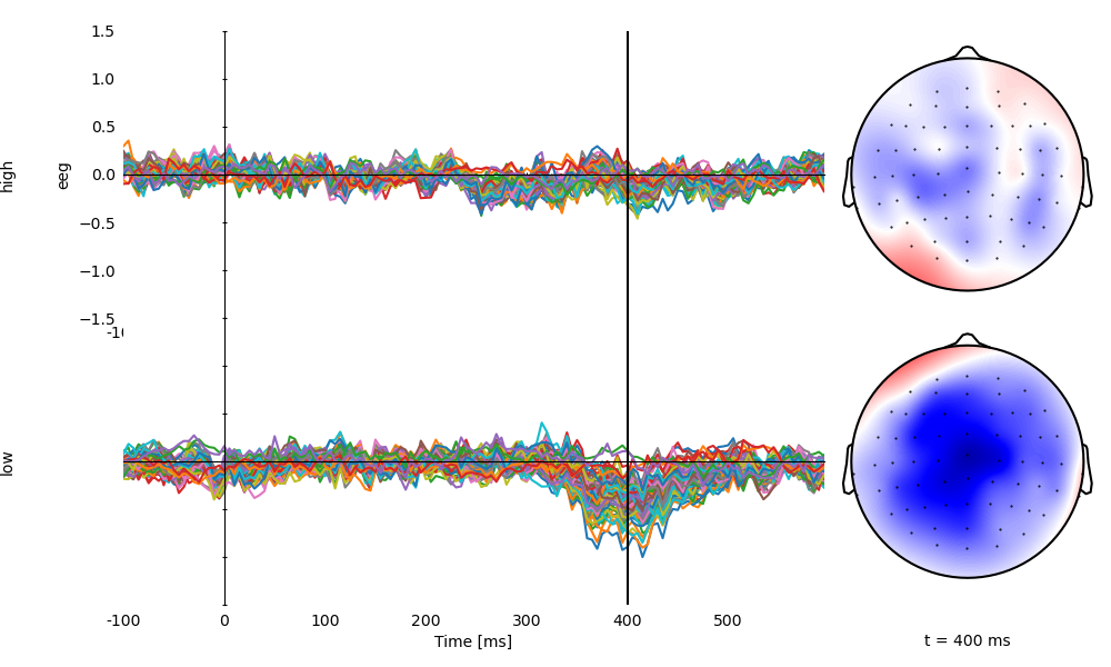
Plot averages separately for high and low cloze

p = plot.TopoButterfly('eeg', 'predictability', data=ds, vmax=1.5, clip='circle', frame='t', axh=3)
p.set_time(0.400)

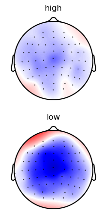
Average over time in the N400 time window

p = plot.Topomap('eeg.mean(time=(0.300, 0.500))', 'predictability', data=ds, vmax=1, clip='circle')

Plot the first 20 trials, labeled with cloze propability

labels = [f'{i} ({c:.2f})' for i, c in enumerate(cloze[:20])]
p = plot.Butterfly('eeg[:20]', '.case', data=ds, axtitle=labels)