Dataset basics

# Author: Christian Brodbeck <christianbrodbeck@nyu.edu>
from eelbrain import *
import numpy

A dataset can be constructed column by column, by adding one variable after another:

# initialize an empty Dataset:
ds = Dataset()
# numeric values are added as Var object:
ds['y'] = Var(numpy.random.normal(0, 1, 6))
# categorical data as represented in Factors:
ds['a'] = Factor(['a', 'b', 'c'], repeat=2)
# A variable that's equal in all cases can be assigned quickly:
ds[:, 'z'] = 0.
# check the result:
ds

#	y	a	z
0	-0.92083	a	0
1	0.33723	a	0
2	-1.2423	b	0
3	-0.67979	b	0
4	0.64146	c	0
5	1.504	c	0

For larger datasets it can be more convenient to print only the first few cases…

ds.head()

#	y	a	z
0	-0.92083	a	0
1	0.33723	a	0
2	-1.2423	b	0
3	-0.67979	b	0
4	0.64146	c	0
5	1.504	c	0

… or a summary of variables:

ds.summary()

Key	Type	Values
y	Var	-1.24233, -0.920828, -0.679789, 0.337232, 0.641463, 1.50401
a	Factor	a:2, b:2, c:2
z	Var	0:6

Dataset: 6 cases

An alternative way of constructing a dataset is case by case (i.e., row by row):

rows = []
for i in range(6):
    subject = f'S{i}'
    y = numpy.random.normal(0, 1)
    a = 'abc'[i % 3]
    rows.append([subject, y, a])
ds = Dataset.from_caselist(['subject', 'y', 'a'], rows, random='subject')
ds

#	subject	y	a
0	S0	0.70615	a
1	S1	1.2669	b
2	S2	-1.0549	c
3	S3	-0.96541	a
4	S4	0.56768	b
5	S5	-0.43722	c

Example

Below is a simple example using data objects (for more, see the Examples):

y = numpy.empty(21)
y[:14] = numpy.random.normal(0, 1, 14)
y[14:] = numpy.random.normal(2, 1, 7)
ds = Dataset({
    'a': Factor('abc', 'A', repeat=7),
    'y': Var(y, 'Y'),
})
ds

#	a	y
0	a	-0.8095
1	a	0.48318
2	a	0.63569
3	a	-2.4486
4	a	0.54863
5	a	0.011343
6	a	0.80284
7	b	-0.72617
8	b	-0.59264
9	b	1.0033
10	b	0.94024
11	b	-0.42219
12	b	1.1817
13	b	0.01647
14	c	1.1617
15	c	0.45187
16	c	1.1425
17	c	3.8858
18	c	2.192
19	c	1.5811
20	c	2.6167

table.frequencies('a', data=ds)

#	a	n
0	a	7
1	b	7
2	c	7

test.ANOVA('y', 'a', data=ds)

	SS	df	MS	F	p
a	15.75	2	7.87	7.06**	.005
Residuals	20.06	18	1.11
Total	35.81	20

test.pairwise('y', 'a', data=ds, corr='Hochberg')

Pairwise T-Tests (independent samples)

	b	c
a	t12 = -0.58 p = .575 pc = .575	t12 = -3.20* p = .008 pc = .027
b		t12 = -3.12* p = .009 pc = .027

(* Corrected after Hochberg, 1988)

t = test.pairwise('y', 'a', data=ds, corr='Hochberg')
print(t.get_tex())

\begin{center}
\begin{tabular}{lll}
\toprule
 & b & c \\
\midrule
a & $t_{12} = -0.58^{   \ \ \ }$\\
$p = .575$\\
$p_{c} = .575$ & $t_{12} = -3.20^{*  \ \ }$\\
$p = .008$\\
$p_{c} = .027$ \\
b &  & $t_{12} = -3.12^{*  \ \ }$\\
$p = .009$\\
$p_{c} = .027$ \\
\bottomrule
\end{tabular}
\end{center}

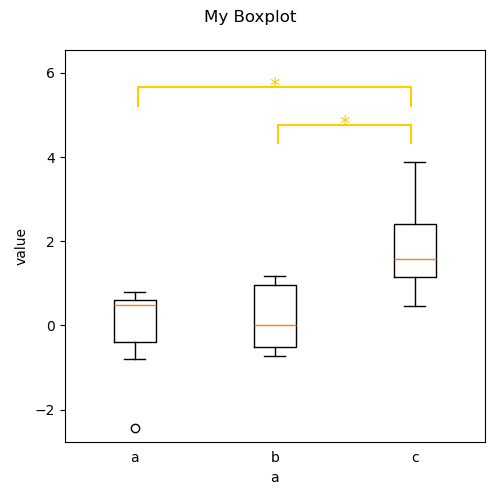
p = plot.Boxplot('y', 'a', data=ds, title="My Boxplot", ylabel="value", corr='Hochberg')