Two-stage test

When trials are associated with continuous predictor variables, averaging is often a poor solution that loses part of the data. In such cases, a two-stage design can be employed that allows using the continuous predictor variable to test hypotheses at the group level. A two-stage analysis involves:

• Stage 1: fit a regression model to each individual subject’s data

• Stage 2: test regression coefficients at the group level

The example uses the same simulated data and design used in Multiple regression. The data are meant to vaguely resemble data from a word reading experiment, but not intended as a physiologically realistic simulation.

# sphinx_gallery_thumbnail_number = 1
from eelbrain import *

Stage 1

Generate simulated data: each function call to datasets.simulate_erp() generates a dataset for one subject (in a real experiment this would be replaced with a function that loads data for this subject). For each subject, a multiple regression model is fit using n characters and cloze probability as continuous predictor variables.

lms = []
for subject in range(10):
    # generate data for one subject
    ds = datasets.simulate_erp(seed=subject)
    # Re-reference EEG data
    ds['eeg'] -= ds['eeg'].mean(sensor=['M1', 'M2'])
    # Fit stage 1 model (samples=0 because we do not need permutations at stage 1)
    lm = testnd.LM('eeg', 'n_chars + cloze', data=ds, samples=0, subject=str(subject))
    lms.append(lm)

Stage 2

Prepare a Dataset with the first level statistic of interest.

rows = []
for lm in lms:
    rows.append([lm.subject, lm.t('intercept'), lm.t('n_chars'), lm.t('cloze')])
# When creating the dataset for stage 2 analysis, declare subject as random factor;
# this is only relevant if performing ANOVA as stage 2 test.
data = Dataset.from_caselist(['subject', 'intercept', 'n_chars', 'cloze'], rows, random='subject')
data

#	subject
0	0
1	1
2	2
3	3
4	4
5	5
6	6
7	7
8	8
9	9

NDVars: intercept, n_chars, cloze

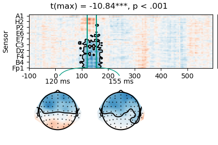
Now we can test whether the first stage estimates are consistent across subject.

result = testnd.TTestOneSample('n_chars', data=data, pmin=0.05, tstart=0, tstop=0.300)
p = plot.TopoArray(result, t=[0.120, 0.155, None], title=result, head_radius=0.35)
p_cb = p.plot_colorbar(right_of=p.axes[0], label='t')

Permutation test:   0%|          | 0/1023 [00:00<?, ? permutations/s]
Permutation test:  21%|██        | 213/1023 [00:00<00:00, 2121.99 permutations/s]
Permutation test:  44%|████▍     | 448/1023 [00:00<00:00, 2250.32 permutations/s]
Permutation test:  67%|██████▋   | 688/1023 [00:00<00:00, 2318.40 permutations/s]
Permutation test:  92%|█████████▏| 940/1023 [00:00<00:00, 2395.42 permutations/s]
Permutation test: 100%|██████████| 1023/1023 [00:00<00:00, 2346.18 permutations/s]

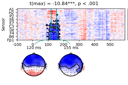
Instead of t-values, we might want to visualize regression coefficients:

rows = []
for lm in lms:
    rows.append([lm.subject, lm.coefficient('n_chars')])
data_c = Dataset.from_caselist(['subject', 'n_chars'], rows, random='subject')

# mask regression coefficients by significance to add outlines to plot
masked_c = data_c['n_chars'].mean('case').mask(result.p > 0.05, missing=True)

p = plot.TopoArray(masked_c, t=[0.120, 0.155, None], title=result, head_radius=0.35)
p_cb = p.plot_colorbar(right_of=p.axes[0], label='µV', unit=1e-6)

Of course, other tests could be applied at stage 2, for example

• T-tests to compare coefficients for two different regressor, or two differen subject groups

• ANOVA for multiple regressors and/or subject groups

• Multiple regression models with subject variables to test for individual differnces