Note
Click here to download the full example code
Compare topographies
This example shows how to compare EEG topographies, based on the method described by McCarthy & Wood 1.
# sphinx_gallery_thumbnail_number = 4
from eelbrain import *
Simulated data
Generate a simulated dataset (as in the Cluster-based permutation t-test example)
dss = []
for subject in range(10):
    # generate data for one subject
    ds = datasets.simulate_erp(seed=subject)
    # average across trials to get condition means
    ds_agg = ds.aggregate('cloze_cat')
    # add the subject name as variable
    ds_agg[:, 'subject'] = f'S{subject:02}'
    dss.append(ds_agg)

ds = combine(dss)
# make subject a random factor (to treat it as random effect for ANOVA)
ds['subject'].random = True
# Re-reference the EEG data (i.e., subtract the mean of the two mastoid channels):
ds['eeg'] -= ds['eeg'].mean(sensor=['M1', 'M2'])
print(ds.head())
Out:
n    cloze     cloze_cat   n_chars   subject
--------------------------------------------
40   0.88051   high        4.125     S00
40   0.17241   low         3.825     S00
40   0.89466   high        4         S01
40   0.13778   low         4.575     S01
40   0.90215   high        4.275     S02
40   0.12206   low         3.9       S02
40   0.88503   high        4         S03
40   0.14273   low         4.175     S03
40   0.90499   high        4.1       S04
40   0.15732   low         3.5       S04
--------------------------------------------
NDVars: eeg
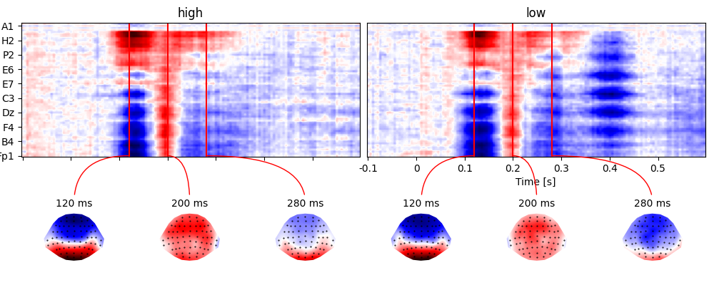
The simulated data in the two conditions:
p = plot.TopoArray('eeg', 'cloze_cat', ds=ds, axh=2, axw=10, t=[0.120, 0.200, 0.280])
Test between conditions
Test whether the 120 ms topography differs between the two cloze conditions. The dataset already includes one row per cell (i.e., per cloze condition and subject). Consequently, we can just index the topography at the desired time point:
topography = ds['eeg'].sub(time=0.120)
# normalize the data in accordance with McCarth & Wood (1985)
topography = normalize_in_cells(topography, 'sensor', 'cloze_cat', ds)
# "melt" the topography NDVar to turn the sensor dimension into a Factor
ds_topography = table.melt_ndvar(topography, 'sensor', ds=ds)
# Note EEG is a single column, and the last column indicates the sensor
ds_topography.head()
Out:
n    cloze     cloze_cat   n_chars   subject   eeg        sensor
----------------------------------------------------------------
40   0.88051   high        4.125     S00       -0.55174   Fp1
40   0.17241   low         3.825     S00       -0.94975   Fp1
40   0.89466   high        4         S01       -1.0303    Fp1
40   0.13778   low         4.575     S01       -1.5701    Fp1
40   0.90215   high        4.275     S02       -1.3857    Fp1
40   0.12206   low         3.9       S02       -1.5753    Fp1
40   0.88503   high        4         S03       -1.1537    Fp1
40   0.14273   low         4.175     S03       -1.6285    Fp1
40   0.90499   high        4.1       S04       -1.9244    Fp1
40   0.15732   low         3.5       S04       -1.5299    Fp1
ANOVA to test whether the effect of cloze_cat differs between sensors:
test.ANOVA('eeg', 'cloze_cat * sensor * subject', ds=ds_topography)
Out:
<ANOVA: eeg ~ cloze_cat + sensor + cloze_cat x sensor + subject + cloze_cat x subject + sensor x subject + cloze_cat x sensor x subject
                            SS     df      MS   MS(denom)   df(denom)           F        p
  ----------------------------------------------------------------------------------------
  cloze_cat              -0.00      1   -0.00        3.64           9    -0.00       1.000
  sensor               1295.07     64   20.24        0.08         576   255.94***   < .001
  cloze_cat x sensor      4.93     64    0.08        0.07         576     1.06        .366
  ----------------------------------------------------------------------------------------
  Total                1468.53   1299
>
The non-significant interaction suggests that the effect of cloze_cat does not differ between sensors, i.e., the topographies do not differ, which is consistent with being generated by the same underlying neural sources.
Test two time points
Since we’re not interested in condition here, we first average across conditions, i.e., with the goal of having one row per subject:
ds_average = ds.aggregate('subject', drop_bad=True)
print(ds_average)
Out:
n    cloze     n_chars   subject
--------------------------------
40   0.52646   3.975     S00
40   0.51622   4.2875    S01
40   0.51211   4.0875    S02
40   0.51388   4.0875    S03
40   0.53115   3.8       S04
40   0.52163   4.0375    S05
40   0.53789   4.2       S06
40   0.52491   4.1125    S07
40   0.52464   4.15      S08
40   0.52559   3.8875    S09
--------------------------------
NDVars: eeg
In order to compare two time points, we need to construct a new dataset with time point as Factor:
dss = []
for time in [0.120, 0.280]:
    ds_time = ds_average['subject',]  # A new dataset with the 'subject' variable only
    ds_time['eeg'] = ds_average['eeg'].sub(time=time)
    ds_time[:, 'time'] = f'{time*1000:.0f} ms'
    dss.append(ds_time)
ds_times = combine(dss)
ds_times.summary()
Out:
Key       Type     Values
------------------------------------------------------------------------------------------------
subject   Factor   S00:2, S01:2, S02:2, S03:2, S04:2, S05:2, S06:2, S07:2, S08:2, S09:2 (random)
eeg       NDVar    65 sensor; -3.62446e-06 - 3.90635e-06
time      Factor   120 ms:10, 280 ms:10
------------------------------------------------------------------------------------------------
None: 20 cases
Then, normalize the data in accordance with McCarth & Wood (1985)
topography = normalize_in_cells('eeg', 'sensor', 'time', ds=ds_times)
# "melt" the topography NDVar to turn the sensor dimension into a Factor
ds_topography = table.melt_ndvar(topography, 'sensor', ds=ds_times)
# Note EEG is a single column, and the last column indicates the sensor
ds_topography.head()
Out:
subject   time     eeg        sensor
------------------------------------
S00       120 ms   -0.74756   Fp1
S01       120 ms   -1.2964    Fp1
S02       120 ms   -1.4811    Fp1
S03       120 ms   -1.3882    Fp1
S04       120 ms   -1.735     Fp1
S05       120 ms   -1.3842    Fp1
S06       120 ms   -1.2591    Fp1
S07       120 ms   -1.3146    Fp1
S08       120 ms   -1.4126    Fp1
S09       120 ms   -1.0279    Fp1
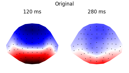
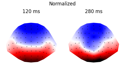
Plot the topographies before and after normalization:
p = plot.Topomap('eeg', 'time', ds=ds_times, ncol=2, title="Original")
p = plot.Topomap(topography, 'time', ds=ds_times, ncol=2, title="Normalized")
Compre the topographies with the ANOVA – test whether the effect of time differs between sensors:
test.ANOVA('eeg', 'time * sensor * subject', ds=ds_topography)
Out:
<ANOVA: eeg ~ time + sensor + time x sensor + subject + time x subject + sensor x subject + time x sensor x subject
                       SS     df      MS   MS(denom)   df(denom)           F        p
  -----------------------------------------------------------------------------------
  time               0.00      1    0.00       12.55           9
  sensor          1269.88     64   19.84        0.19         576   105.37***   < .001
  time x sensor     30.12     64    0.47        0.18         576     2.57***   < .001
  -----------------------------------------------------------------------------------
  Total           1754.93   1299
>
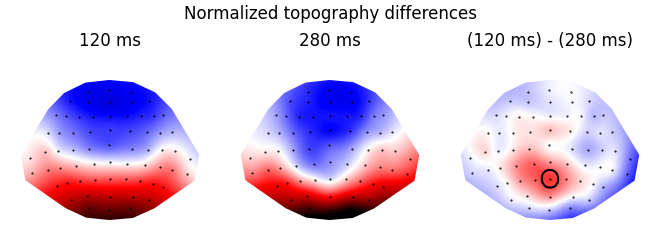
Visualize the difference
res = testnd.TTestRelated(topography, 'time', match='subject', ds=ds_times)
p = plot.Topomap(res, ncol=3, title="Normalized topography differences")
References
- 1
McCarthy, G., & Wood, C. C. (1985). Scalp Distributions of Event-Related Potentials—An Ambiguity Associated with Analysis of Variance Models. Electroencephalography and Clinical Neurophysiology, 61, S226–S227. 10.1016/0013-4694(85)90858-2
Total running time of the script: ( 0 minutes 13.670 seconds)