Introduction

Data are represented with there primary data-objects:

• Factor for categorial variables

• Var for scalar variables

• NDVar for multidimensional data (e.g. a variable measured at different time points)

Multiple variables belonging to the same dataset can be grouped in a Dataset object.

Factor

A Factor is a container for one-dimensional, categorial data: Each case is described by a string label. The most obvious way to initialize a Factor is a list of strings:

# sphinx_gallery_thumbnail_number = 3
from eelbrain import *

a = Factor(['a', 'a', 'a', 'a', 'b', 'b', 'b', 'b'], name='A')
a

Factor(['a', 'a', 'a', 'a', 'b', 'b', 'b', 'b'], name='A')

Since Factor initialization simply iterates over the given data, the same Factor could be initialized with:

a = Factor('aaaabbbb', name='A')
a

Factor(['a', 'a', 'a', 'a', 'b', 'b', 'b', 'b'], name='A')

There are other shortcuts to initialize factors (see also the Factor class documentation):

a = Factor(['a', 'b', 'c'], repeat=4, name='A')
a

Factor(['a', 'a', 'a', 'a', 'b', 'b', 'b', 'b', 'c', 'c', 'c', 'c'], name='A')

Indexing works like for arrays:

a[0]

'a'

a[0:6]

Factor(['a', 'a', 'a', 'a', 'b', 'b'], name='A')

All values present in a Factor are accessible in its Factor.cells attribute:

a.cells

('a', 'b', 'c')

Based on the Factor’s cell values, boolean indexes can be generated:

a == 'a'

array([ True,  True,  True,  True, False, False, False, False, False,
       False, False, False])

a.isany('a', 'b')

array([ True,  True,  True,  True,  True,  True,  True,  True, False,
       False, False, False])

a.isnot('a', 'b')

array([False, False, False, False, False, False, False, False,  True,
        True,  True,  True])

Interaction effects can be constructed from multiple factors with the % operator:

b = Factor(['d', 'e'], repeat=2, tile=3, name='B')
b

Factor(['d', 'd', 'e', 'e', 'd', 'd', 'e', 'e', 'd', 'd', 'e', 'e'], name='B')

i = a % b
i

A % B

Interaction effects are in many ways interchangeable with factors in places where a categorial model is required:

i.cells

(('a', 'd'), ('a', 'e'), ('b', 'd'), ('b', 'e'), ('c', 'd'), ('c', 'e'))

i == ('a', 'd')

array([ True,  True, False, False, False, False, False, False, False,
       False, False, False])

Var

The Var class is a container for one-dimensional numpy.ndarray:

y = Var([1, 2, 3, 4, 5, 6])
y

Var([1, 2, 3, 4, 5, 6])

Indexing works as for factors

y[5]

6

y[2:]

Var([3, 4, 5, 6])

Many array operations can be performed on the object directly

y + 1

Var([2, 3, 4, 5, 6, 7])

For any more complex operations the corresponding numpy.ndarray can be retrieved in the Var.x attribute:

y.x

array([1, 2, 3, 4, 5, 6])

Note

The Var.x attribute is not intended to be replaced; rather, a new Var object should be created for a new array.

NDVar

NDVar objects are containers for multidimensional data, and manage the description of the dimensions along with the data. NDVar objects are usually constructed automatically by an importer function (see File I/O), for example by importing data from MNE-Python through load.mne.

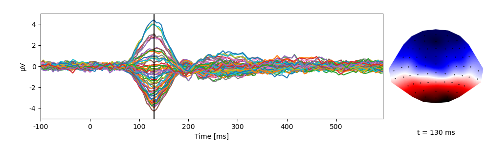
Here we use data from a simulated EEG experiment as example:

data = datasets.simulate_erp(snr=0.5)
eeg = data['eeg']
eeg

<NDVar 'eeg': 80 case, 140 time, 65 sensor>

This representation shows that eeg contains 80 trials of data (cases), with 140 time points and 35 EEG sensors.

The object provides access to the underlying array…

eeg.x

array([[[-1.10225035e-07, -1.21398829e-06,  1.35355502e-06, ...,
         -6.12893745e-07, -2.51649218e-06, -1.33879697e-06],
        [ 1.03057616e-06, -1.97609123e-06,  5.55910753e-08, ...,
         -1.75102062e-06, -6.06858438e-06, -1.48262419e-06],
        [ 2.26162309e-06, -2.76452386e-06, -1.64393195e-06, ...,
         -2.56737373e-06, -3.39503569e-06, -1.77351586e-06],
        ...,
        [ 1.27928669e-06, -2.54650493e-06, -1.43902791e-06, ...,
         -1.14332247e-06, -7.59471495e-07, -1.39821309e-06],
        [ 5.83282737e-07, -2.50177953e-06, -1.96916415e-06, ...,
         -1.70881189e-07, -1.97792491e-06,  7.97185353e-07],
        [ 1.00898892e-06, -2.53987234e-06, -6.87119668e-07, ...,
          1.88518585e-06, -2.40118283e-06,  2.64689298e-06]],

       [[ 7.91017764e-07,  7.71971488e-07,  1.30305895e-06, ...,
         -4.75553281e-06, -5.09520252e-07, -6.73740855e-06],
        [ 1.87471343e-06,  1.10809976e-06,  1.42277977e-06, ...,
         -2.39445056e-06,  2.08157541e-06, -3.53570199e-06],
        [ 3.62235228e-06,  7.41319898e-07, -3.49176708e-07, ...,
         -2.82527907e-06, -8.71546782e-07, -3.88825269e-06],
        ...,
        [ 4.11020044e-07,  2.53134557e-06,  2.02588775e-06, ...,
          1.63371394e-06,  1.75639879e-06, -3.22866969e-07],
        [-8.12184975e-08,  1.19783257e-08,  1.19906259e-06, ...,
          1.12612937e-06, -2.73425855e-06, -1.50807251e-08],
        [-1.48969900e-07,  1.02379750e-06,  1.90242890e-07, ...,
         -9.31770169e-07,  3.19786912e-07, -1.57491654e-06]],

       [[-5.70450429e-07,  2.12182688e-06, -5.69412054e-07, ...,
          2.37708527e-06,  9.37329957e-07,  2.78432254e-06],
        [-7.37623648e-07,  2.72325232e-06, -1.96874417e-07, ...,
          2.58707902e-06, -8.01410389e-08,  2.32243357e-06],
        [-1.58156464e-06,  2.49840962e-06, -9.17596458e-07, ...,
          1.39761570e-07, -1.76330512e-07,  5.79787961e-07],
        ...,
        [-2.38621266e-06, -8.99388305e-07, -2.34086858e-06, ...,
          4.76447796e-06,  2.63580832e-06,  4.52300984e-06],
        [-1.04528612e-06, -4.22921727e-07, -1.40656041e-06, ...,
          4.72477781e-06, -1.05594628e-06,  4.79468728e-06],
        [-1.39863144e-06, -3.56393153e-07, -1.70212073e-06, ...,
          3.42515240e-06, -1.34744634e-06,  4.70863707e-06]],

       ...,

       [[-1.86308732e-06,  3.40093890e-07,  4.05648389e-07, ...,
         -2.85624522e-06,  8.61272186e-08, -5.85148186e-06],
        [-1.24991478e-06,  1.10403278e-06,  2.11822745e-06, ...,
         -6.68324617e-08,  1.03962727e-06, -2.65518697e-06],
        [-6.01251125e-07, -1.02557637e-06, -9.88862751e-07, ...,
          1.19219068e-06,  4.49834173e-06, -1.45729409e-06],
        ...,
        [-2.60819856e-06, -1.14139878e-06, -2.32209565e-07, ...,
          2.28403104e-06,  7.43478658e-06,  6.45469349e-07],
        [-1.77894845e-06, -3.29765670e-06, -1.96107364e-07, ...,
          3.17559439e-06,  8.82660892e-07,  1.14646057e-06],
        [-4.46974178e-07, -1.49241340e-06, -9.91849226e-07, ...,
          1.50548785e-06,  4.02040655e-06, -7.80036576e-07]],

       [[-2.58927496e-06, -6.42217652e-07, -6.51667051e-07, ...,
          1.39914167e-06,  1.07433007e-06,  4.62944481e-07],
        [ 8.39045230e-07,  1.35565975e-06,  2.19848898e-06, ...,
         -1.84449635e-07,  3.03922516e-07, -6.40152619e-07],
        [ 2.03991426e-06,  2.96032981e-06,  1.86645511e-06, ...,
          1.14277459e-06, -2.05518754e-06,  7.61602543e-07],
        ...,
        [ 1.10087279e-06,  3.53600540e-06,  3.89314588e-06, ...,
         -1.54317240e-06,  1.32320950e-06, -2.62412434e-06],
        [-4.13975079e-07,  2.61693672e-06,  9.21826295e-07, ...,
          4.31760530e-07,  2.19988807e-08,  3.86507114e-07],
        [ 5.69702800e-07,  3.26813717e-06,  1.76872363e-06, ...,
         -1.34588335e-06, -4.98871043e-07, -2.59585280e-06]],

       [[-1.08671813e-06,  1.68348411e-06,  8.88593660e-07, ...,
          4.36248556e-06,  1.79194589e-06,  4.90462425e-06],
        [-1.70646054e-06,  9.60379945e-07,  4.99692848e-07, ...,
          5.04600076e-06,  3.50628649e-06,  7.49790857e-06],
        [-5.89765709e-07,  2.06204158e-07, -4.52929175e-07, ...,
          4.39870762e-06,  3.38398127e-06,  5.63799640e-06],
        ...,
        [ 1.09576534e-06,  1.18006051e-06,  9.58097062e-07, ...,
          2.56989150e-06,  2.55069701e-06,  4.85468318e-06],
        [-9.09168160e-07, -1.24791905e-06, -1.05919818e-06, ...,
          4.43486532e-06,  4.98945467e-06,  4.77573354e-06],
        [-2.84420080e-06, -5.57317398e-07, -1.55925347e-06, ...,
          5.27693951e-06,  1.42830967e-06,  4.90967646e-06]]])

… and dimension descriptions:

eeg.sensor

<Sensor n=65, name='standard_alphabetic'>

eeg.time

UTS(-0.1, 0.005, 140)

Eelbrain functions take advantage of the dimensions descriptions (such as sensor locations), for example for plotting:

p = plot.TopoButterfly(eeg, t=0.130)

NDVar offer functionality similar to numpy.ndarray, but take into account the properties of the dimensions. For example, through the NDVar.sub() method, indexing can be done using meaningful descriptions, such as indexing a time slice in seconds …

eeg_130 = eeg.sub(time=0.130)
p = plot.Topomap(eeg_130)
eeg_130

<NDVar 'eeg': 80 case, 65 sensor>

… or extracting data from a specific sensor:

eeg_fz = eeg.sub(sensor='Fz')
p = plot.UTSStat(eeg_fz)
eeg_fz

<NDVar 'eeg': 80 case, 140 time>

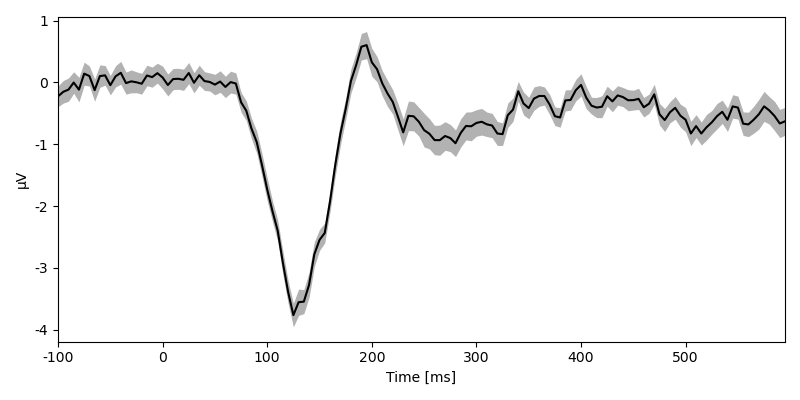
Other methods allow aggregating data, for example an RMS over sensor …

eeg_rms = eeg.rms('sensor')
plot.UTSStat(eeg_rms)
eeg_rms

<NDVar 'eeg': 80 case, 140 time>

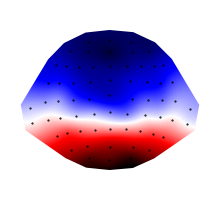
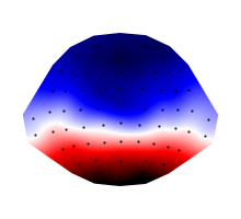
… or a mean in a time window:

eeg_average = eeg.mean(time=(0.100, 0.150))
p = plot.Topomap(eeg_average)

Dataset

A Dataset is a container for multiple variables (Factor, Var and NDVar) that describe the same cases. It can be thought of as a data table with columns corresponding to different variables and rows to different cases. Consider the dataset containing the simulated EEG data used above:

data

cloze	predictability	n_chars
0.026139	low	4
0.99529	high	5
0.93062	high	3
0.82404	high	7
0.17041	low	4
0.18508	low	4
0.23345	low	4
0.80784	high	3
0.24979	low	7
0.26753	low	4
0.19377	low	5
0.13128	low	5
0.11503	low	3
0.1244	low	4
0.94785	high	5
0.17053	low	6
0.84889	high	7
0.20455	low	3
0.21456	low	5
0.89373	high	4
0.23416	low	6
0.85923	high	6
0.23975	low	5
0.82375	high	4
0.82579	high	3
0.92097	high	7
0.19198	low	4
0.93413	high	5
0.13844	low	3
0.15655	low	4
0.81922	high	3
0.93335	high	4
0.96759	high	6
0.1271	low	7
0.82208	high	6
0.99535	high	4
0.86309	high	5
0.87274	high	4
0.043006	low	4
0.83226	high	4
0.23227	low	5
0.85066	high	6
0.2891	low	7
0.82041	high	5
0.99767	high	5
0.9642	high	6
0.0056369	low	5
0.83179	high	3
0.16346	low	6
0.83932	high	7
0.035482	low	4
0.079367	low	6
0.27768	low	6
0.8719	high	6
0.82764	high	7
0.93953	high	5
0.85656	high	4
0.261	low	4
0.28312	low	4
0.16464	low	5
0.84178	high	5
0.13685	low	7
0.0060655	low	6
0.88772	high	3
0.18083	low	3
0.15867	low	5
0.81205	high	7
0.23752	low	7
0.18363	low	5
0.87375	high	5
0.89326	high	6
0.88741	high	6
0.021311	low	5
0.2834	low	6
0.91404	high	5
0.29359	low	6
0.84208	high	5
0.81942	high	5
0.18529	low	7
0.93127	high	4

NDVars: eeg

Because this can be more output than needed, the Dataset.head() method only shows the first couple of rows:

data.head()

cloze	predictability	n_chars
0.026139	low	4
0.99529	high	5
0.93062	high	3
0.82404	high	7
0.17041	low	4
0.18508	low	4
0.23345	low	4
0.80784	high	3
0.24979	low	7
0.26753	low	4

NDVars: eeg

This dataset containes severeal univariate columns: cloze, predictability, and n_chars. The last line also indicates that the dataset contains an NDVar called eeg. The NDVar is not displayed as column because it contains many values per row. In the NDVar, the Case dimension corresponds to the row in the dataset (which here corresponds to simulated trial number):

data['eeg']

<NDVar 'eeg': 80 case, 140 time, 65 sensor>

The type and value range of each entry in the Dataset can be shown using the Dataset.summary() method:

data.summary()

Key	Type	Values
eeg	NDVar	140 time, 65 sensor; -1.11871e-05 - 1.11083e-05
cloze	Var	0.00563694 - 0.997675
predictability	Factor	high:40, low:40
n_chars	Var	3:10, 4:20, 5:22, 6:16, 7:12

Dataset: 80 cases

An even shorter summary can be generated by the string representation:

repr(data)

"<Dataset (80 cases) 'eeg':Vnd, 'cloze':V, 'predictability':F, 'n_chars':V>"

Here, 80 cases indicates that the Dataset contains 80 rows. The subsequent dictionary-like representation shows the keys and the types of the corresponding values (F: Factor, V: Var, Vnd: NDVar).

Datasets can be indexed with columnn names, …

data['cloze']

Var([0.0261388, 0.995292, 0.930622, 0.824039, 0.170413, 0.18508, 0.233447, 0.807838, 0.249786, 0.267532, 0.193768, 0.131276, 0.115032, 0.124399, 0.947853, 0.17053, 0.848885, 0.204546, 0.214557, 0.89373, 0.234159, 0.859228, 0.239748, 0.823746, 0.825785, 0.920969, 0.191976, 0.934128, 0.138444, 0.156554, 0.81922, 0.933353, 0.967589, 0.127096, 0.822075, 0.995352, 0.863086, 0.872742, 0.043006, 0.832262, 0.23227, 0.850658, 0.289099, 0.820409, 0.997675, 0.964199, 0.00563694, 0.831794, 0.163465, 0.839316, 0.0354823, 0.0793667, 0.277679, 0.871902, 0.827637, 0.939526, 0.856561, 0.261004, 0.283124, 0.164644, 0.841775, 0.136845, 0.00606552, 0.88772, 0.180829, 0.158668, 0.812045, 0.237518, 0.183629, 0.873745, 0.893262, 0.887406, 0.0213108, 0.283401, 0.914039, 0.293586, 0.842077, 0.81942, 0.185291, 0.931266], name='cloze')

… row numbers, …

data[2:5]

cloze	predictability	n_chars
0.93062	high	3
0.82404	high	7
0.17041	low	4

NDVars: eeg

… or both, in wich case row comes before column:

data[2:5, 'n_chars']

Var([3, 7, 4], name='n_chars')

Array-based indexing also allows indexing based on the Dataset’s variables:

data['n_chars'] == 3

array([False, False,  True, False, False, False, False,  True, False,
       False, False, False,  True, False, False, False, False,  True,
       False, False, False, False, False, False,  True, False, False,
       False,  True, False,  True, False, False, False, False, False,
       False, False, False, False, False, False, False, False, False,
       False, False,  True, False, False, False, False, False, False,
       False, False, False, False, False, False, False, False, False,
        True,  True, False, False, False, False, False, False, False,
       False, False, False, False, False, False, False, False])

data[data['n_chars'] == 3]

cloze	predictability	n_chars
0.93062	high	3
0.80784	high	3
0.11503	low	3
0.20455	low	3
0.82579	high	3
0.13844	low	3
0.81922	high	3
0.83179	high	3
0.88772	high	3
0.18083	low	3

NDVars: eeg

Dataset.eval() allows evaluatuing code strings in the namespace defined by the dataset, which means that dataset variables can be invoked with just their name:

data.eval("predictability == 'high'")

array([False,  True,  True,  True, False, False, False,  True, False,
       False, False, False, False, False,  True, False,  True, False,
       False,  True, False,  True, False,  True,  True,  True, False,
        True, False, False,  True,  True,  True, False,  True,  True,
        True,  True, False,  True, False,  True, False,  True,  True,
        True, False,  True, False,  True, False, False, False,  True,
        True,  True,  True, False, False, False,  True, False, False,
        True, False, False,  True, False, False,  True,  True,  True,
       False, False,  True, False,  True,  True, False,  True])

Many dataset methods allow using code strings as shortcuts for expressions involving dataset variables, for example indexing:

data.sub("predictability == 'high'").head()

cloze	predictability	n_chars
0.99529	high	5
0.93062	high	3
0.82404	high	7
0.80784	high	3
0.94785	high	5
0.84889	high	7
0.89373	high	4
0.85923	high	6
0.82375	high	4
0.82579	high	3

NDVars: eeg

Columns in the Dataset can be used to define models, for statistics, aggregating and plotting. Any string specified as argument in those functions will be evaluated in the dataset, thuse, because we can use:

data.eval("eeg.sub(sensor='Cz')")

<NDVar 'eeg': 80 case, 140 time>

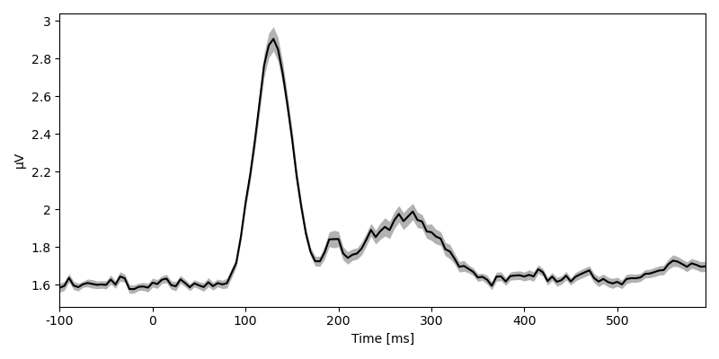
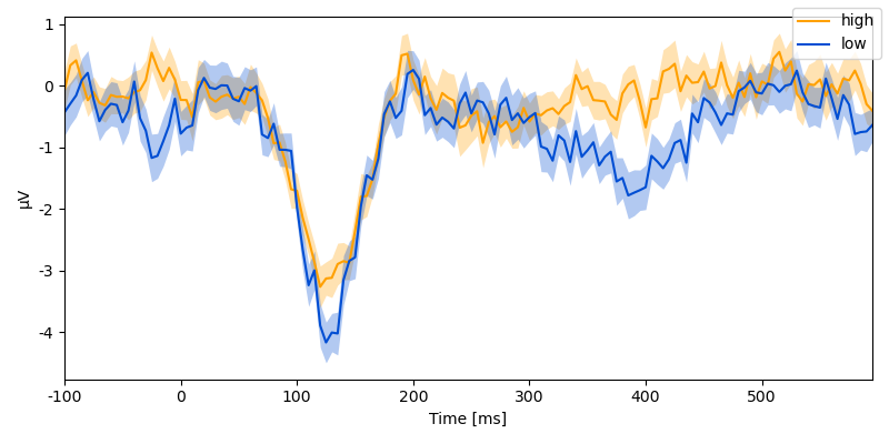
… we can quickly plot the time course of a sensor by condition:

p = plot.UTSStat("eeg.sub(sensor='Cz')", "predictability", data=data)

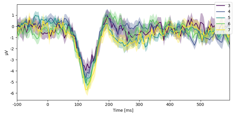
p = plot.UTSStat("eeg.sub(sensor='Fz')", "n_chars", data=data, colors='viridis')

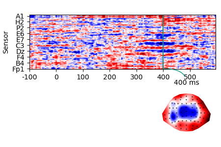
Or calculate a difference wave:

data_average = data.aggregate('predictability')
data_average

n	cloze	predictability	n_chars
40	0.88051	high	5
40	0.17241	low	5

NDVars: eeg

difference = data_average[1, 'eeg'] - data_average[0, 'eeg']
p = plot.TopoArray(difference, t=[None, None, 0.400])

For examples of how to construct datasets from scratch see Dataset basics.