Introduction to Temporal Response Functions (TRFs)

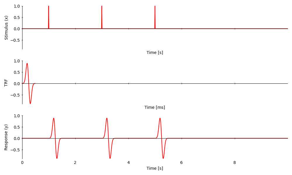
A Temporal Response Function (TRF) is a linear stimulus-response model. The predicted response is a linear convolution of the stimulus with the TRF. A simple illustration of this is that every impulse in the stimulus is associated with a corresponding response, shaped like the TRF:

from eelbrain import *
import numpy as np

# Construct a 10 s long stimulus
time = UTS(0, 0.01, 1000)
x = NDVar(np.zeros(len(time)), time)
# add a few impulses
x[1] = 1
x[3] = 1
x[5] = 1

# Construct a TRF of length 500 ms
trf_time = UTS(0, 0.01, 50)
trf = gaussian(0.200, 0.050, trf_time) - gaussian(0.300, 0.050, trf_time)

# The response is the convolution of the stimulus with the TRF
y = convolve(trf, x)

plot_args = dict(columns=1, axh=2, w=10, frame='t', legend=False, colors='r')
p = plot.UTS([x, trf, y], ylabel=['Stimulus (x)', 'TRF', 'Response (y)'], **plot_args)

Because the convolution is linear:

• Scaled stimuli cause scaled responses

• Overlapping responses add up

x[2] = 0.66
x[5.2] = 1
x[7] = 0.8
x[7.2] = 0.3
x[8.8] = 0.2
x[9] = 0.5
x[9.2] = 0.7

y = convolve(trf, x)
p = plot.UTS([x, trf, y], ylabel=['Stimulus (x)', 'TRF', 'Response (y)'], **plot_args)

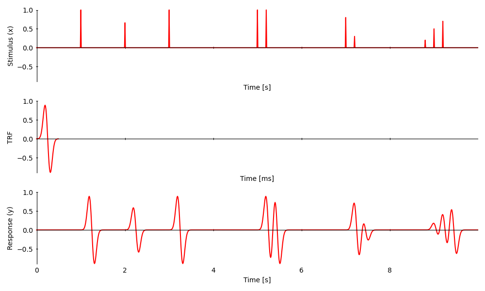
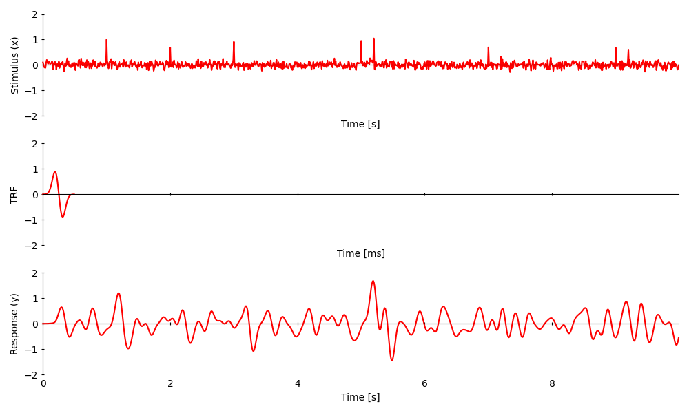
When the stimulus contains only non-zero elements this works just the same, but the TRF shape may not be apparent in the response anymore:

x += np.random.normal(0, 0.1, x.shape)
filter_data(x, 1, 40)
y = convolve(trf, x)
p = plot.UTS([x, trf, y], ylabel=['Stimulus (x)', 'TRF', 'Response (y)'], **plot_args)

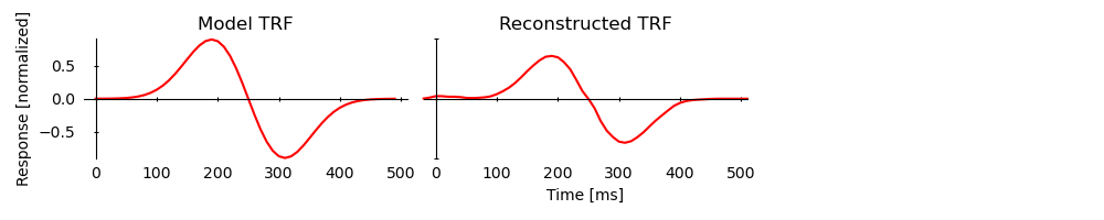
Given a stimulus and a response, there are different methods to reconstruct the TRF. Eelbrain comes with an implementation of boosting(), a coordinate descent algorithm with early stopping based on cross-validation:

fit = boosting(y, x, 0.000, 0.500, basis=0.050, partitions=2)
plot_args = {**plot_args, 'columns': 3}
p = plot.UTS([trf, fit.h, None], axtitle=["Model TRF", "Reconstructed TRF"], **plot_args)