Note
Go to the end to download the full example code.
TRF for Alice EEG Dataset
Estimate a TRF,
starting with a *-raw.fif EEG file and stimulus *.wav files.
The data used is one subject from the Alice dataset. This assumes that the Alice dataset has already been downloded (see the repository readme).
# sphinx_gallery_thumbnail_number = 6
import eelbrain
import eelbrain.datasets._alice
from matplotlib import pyplot
import mne


# Define the dataset root; this will use ~/Data/Alice, replace it with the
# proper path if you downloaded the dataset in a different location
DATA_ROOT = eelbrain.datasets._alice.get_alice_path()

# Define some paths that will be used throughout
STIMULUS_DIR = DATA_ROOT / 'stimuli'
EEG_DIR = DATA_ROOT / 'eeg'

# Load one subject's raw EEG file
SUBJECT = 'S18'
LOW_FREQUENCY = 0.5
HIGH_FREQUENCY = 20
Load EEG data
This section loads EEG data from one subject from the Alice dataset.
raw = mne.io.read_raw(EEG_DIR / SUBJECT / f'{SUBJECT}_alice-raw.fif', preload=True)

# Filter the raw data to the desired band
raw.filter(LOW_FREQUENCY, HIGH_FREQUENCY, n_jobs=1)

# Interpolate bad channels
# This is not structly necessary for a single subject.
# However, when processing multiple subjects, it will allow comparing results across all sensors.
raw.interpolate_bads()

# Load the events embedded in the raw file as eelbrain.Dataset, a type of object that represents a data-table
events = eelbrain.load.mne.events(raw)

# Display the events table:
events
Plot the first 5 seconds of the first trial
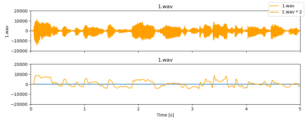
Create a predictor
# Load the sound file corresponding to trigger 1
wav = eelbrain.load.wav(STIMULUS_DIR / f'1.wav')

# Compute the acoustic envelope
envelope = wav.envelope()

# Filter the envelope with the same parameters as the EEG data
envelope = eelbrain.filter_data(envelope, LOW_FREQUENCY, HIGH_FREQUENCY, pad='reflect')
envelope = eelbrain.resample(envelope, 100)

# Visualize the first 5 seconds
p = eelbrain.plot.UTS([wav, envelope * 2], axh=2, w=10, columns=1, xlim=5)

# Add y=0 as reference
p.add_hline(0, zorder=0)
Generate the acoustic envelope for all trials in this dataset
envelopes = []
for stimulus_id in events['event']:
    wav = eelbrain.load.wav(STIMULUS_DIR / f'{stimulus_id}.wav')
    envelope = wav.envelope()
    envelope = eelbrain.filter_data(envelope, LOW_FREQUENCY, HIGH_FREQUENCY, pad='reflect')
    envelope = eelbrain.resample(envelope, 100)
    envelopes.append(envelope)

# Add the envelopes to the events table
events['envelope'] = envelopes

# Add a second predictor corresponding to acoustic onsets
events['onsets'] = [envelope.diff('time').clip(0) for envelope in envelopes]
events
Add EEG trial data
Add EEG data for each trial. We specifically need the EEG data corresponding to each stimulus. Given that each stimulus had a slightly different duration, we need to extract EEG segments that are trimmed differently for each trial.
# Extract the stimulus duration (in seconds) from the envelopes
events['duration'] = eelbrain.Var([envelope.time.tstop for envelope in events['envelope']])
events
Extract EEG data corresponding exactly to the timing of the envelopes
events['eeg'] = eelbrain.load.mne.variable_length_epochs(events, 0, tstop='duration', decim=5, adjacency='auto')
events
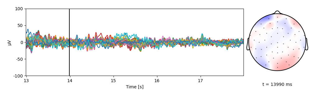
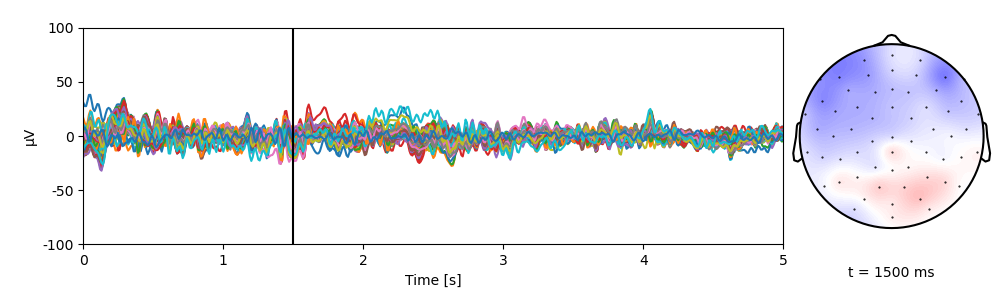
Plot the first 5 seconds of EEG of the first trial (compare above)
p = eelbrain.plot.TopoButterfly(events[0, 'eeg'], t=1.5, xlim=5, vmax=1e-4, h=3, w=10, clip='circle')
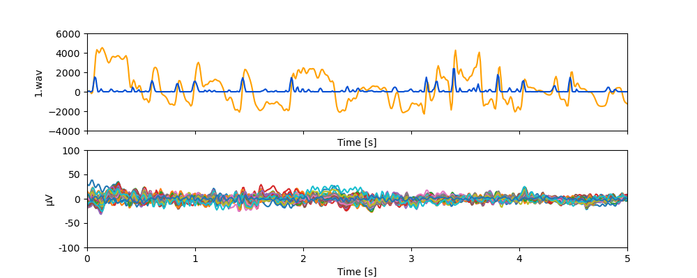
Plot EEG alongside the representations of the sound that was presented
TRF
Estimate the brain’s response function to acoustic onsets.
trf = eelbrain.boosting('eeg', 'onsets', -0.100, 0.500, data=events, basis=0.050, partitions=4)
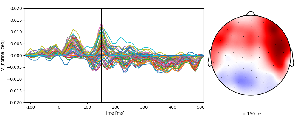
Plot the TRF, highlighting the topography at the global field power maximum
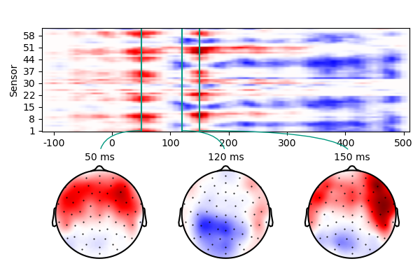
Alternative visualization as array image
p = eelbrain.plot.TopoArray(trf.h, t=[0.050, 0.120, 0.150], w=6, h=4, clip='circle')
Predictive power
In order to derive an unbiased estimate of predictive power,
we can use cross-validation.
That means part of the data is never used while estimating the TRF,
and can be used in the end to calculate how well the TRF can predict neural data.
The boosting() function uses K-fold cross-validation.
Cross-validation is enabled with the test=True parameter,
and K is set through the partitions parameter.
trf_cv = eelbrain.boosting('eeg', 'onsets', 0, 0.500, data=events, basis=0.050, partitions=4, test=True)
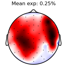
Plot the predictive power across sensors, including the average across all sensors in each figure title.
title = f"Mean exp: {trf_cv.proportion_explained.mean('sensor'):.2%}"
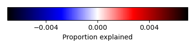
p = eelbrain.plot.Topomap(trf_cv.proportion_explained, clip='circle', title=title)
pcb = p.plot_colorbar('Proportion explained')
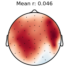
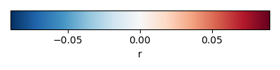
title = f"Mean r: {trf_cv.r.mean('sensor'):.2}"
p = eelbrain.plot.Topomap(trf_cv.r, clip='circle', title=title)
pcb = p.plot_colorbar()
Decoding
Train an envelope decoder on the first 11 trials and use it to decode the envelope of the last trial.
# Use a larger delta to speed up training
decoder = eelbrain.boosting('envelope', 'eeg', -0.500, 0, data=events[:11], partitions=5, delta=0.05)
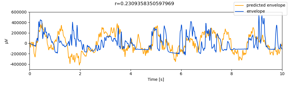
Now use the decoder to reconstruct the envelope of the last trial. Note that,
when using the convolve() function, the time alignment is
handled automatically because the kernel, decoder.h, includes a time axis
(decoder.h.time) with relative delays between input and output.
# Normalize the EEG
eeg_11 = events[11, 'eeg'] / decoder.x_scale

# Predict the envelope by convolving the decoder with the EEG
y_pred = eelbrain.convolve(decoder.h, eeg_11, name='predicted envelope')
Extract the actual envelope and adjust the scale for visualization
y = events[11, 'envelope']
y = y - decoder.y_mean
y /= decoder.y_scale / y_pred.std()
y.name = 'envelope'

r = eelbrain.correlation_coefficient(y, y_pred)
p = eelbrain.plot.UTS([[y_pred, y]], w=10, h=3, xlim=10, title=f"{r=}")
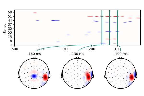
Visualize the decoder weights
p = eelbrain.plot.TopoArray(decoder.h, w=6, h=4, clip='circle', t=[-0.160, -0.130, -0.100])
Total running time of the script: (0 minutes 50.695 seconds)