Volume source space

Basic analysis of volume source space vector data.

Dataset

Load the mne sample data with responses to tones. Data contains multiple trials for a single subject, with tones presented to the left or right ear:

# sphinx_gallery_thumbnail_number = 2
# dataset: mne_sample

from pathlib import Path

from eelbrain import *
import mne


# Load the dataset
data = datasets.get_mne_sample(src='vol', ori='vector')
data.head()

#	i_start	trigger	index	condition	side	modality
0	6994	2	0	RA	R	A
1	7192	1	2	LA	L	A
2	7413	2	4	RA	R	A
3	7612	1	6	LA	L	A
4	7810	2	8	RA	R	A
5	8025	1	10	LA	L	A
6	8233	2	12	RA	R	A
7	8428	1	14	LA	L	A
8	8633	2	16	RA	R	A
9	8857	1	19	LA	L	A

NDVars: src

One-sample test

A one-sample test can be used to detect significant activations. Perform a one-sample test on the right-ear trials only:

result = testnd.Vector('src', sub="side == 'R'", data=data, samples=250, tfce=True, tstart=0.05, tstop=0.200)

Morph the data to the template brain for anatomical visualization.

# Store the test result as NDVar
y = result.masked_difference()

# Make sure the source space for fsaverage exists
fname_src_fsaverage = Path(y.source.subjects_dir) / "fsaverage" / "bem" / "fsaverage-vol-7-src.fif"
if fname_src_fsaverage.exists():
    src_fs = mne.read_source_spaces(fname_src_fsaverage)
else:
    src_fs = mne.setup_volume_source_space('fsaverage', 7, subjects_dir=y.source.subjects_dir)
    src_fs.save(Path(y.source.subjects_dir) / "fsaverage" / "bem" / "fsaverage-vol-7-src.fif")

# Compute the transformation from the sample subject to fsaverage
morph = mne.compute_source_morph(
    y.source.get_source_space(),
    subject_from=y.source.subject,
    subjects_dir=y.source.subjects_dir,
    niter_affine=[10, 10, 5],
    niter_sdr=[10, 10, 5],  # just for speed
    src_to=src_fs,
)

# Morph the test result
y = morph_source_space(y, 'fsaverage', morph=morph)

[2026-05-19 11:06:53][dipy] INFO: ➞ Running center_of_mass step from affine registration...
[2026-05-19 11:06:53][dipy] INFO: ➞ Running translation step from affine registration...
[2026-05-19 11:06:54][dipy] INFO: ➞ Running rigid step from affine registration...
[2026-05-19 11:06:54][dipy] INFO: ➞ Running affine step from affine registration...
[2026-05-19 11:06:54][dipy] INFO: Creating scale space from the moving image. Levels: 3. Sigma factor: 0.200000.
[2026-05-19 11:06:54][dipy] INFO: Creating scale space from the static image. Levels: 3. Sigma factor: 0.200000.
[2026-05-19 11:06:54][dipy] INFO: Optimizing level 2
[2026-05-19 11:06:54][dipy] INFO: Optimizing level 1
[2026-05-19 11:06:54][dipy] INFO: Optimizing level 0

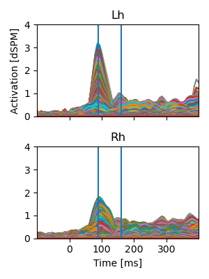
For static visualization, we can use a combination of plot.Butterfly and plot.GlassBrain plots. A plot.Butterfly plot can give a quick overview of amplitudes over time:

# Extract vector norm (amplitude)
y_norm = y.norm('space')
# Split data by hemisphere
butterfly_data = [y_norm.sub(source=hemi, name=hemi.capitalize()) for hemi in ['lh', 'rh']]
# Buterfly plot
p = plot.Butterfly(butterfly_data, axh=2, axw=3)
# Mark time points for anatomical visualization
times = [0.090, 0.160]
for t in times:
    p.add_vline(t)

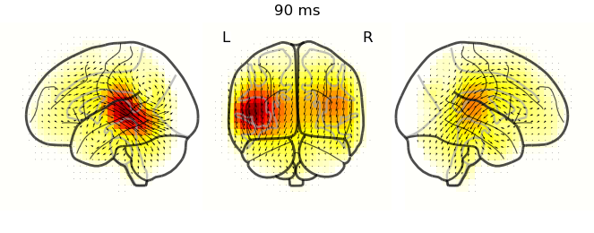
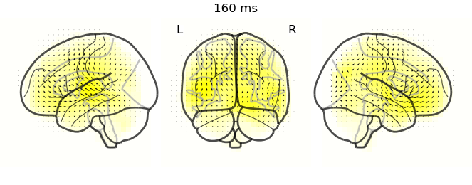
plot.GlassBrain plots show anatomical distribution of activity at relevant time points. Glassbrains project activity through the head, i.e., each voxel in a projection shows the largest value along the line of sight. By comparing different projections, the 3D distribution of activity can be inferred. Here, the lateral view shows activity in temporal regions over auditory cortex, while the coronal view shows how lateral/medial the peaks are:

for t in times:
    p = plot.GlassBrain(y.sub(time=t), title=f"{t * 1000:.0f} ms", vmax=4)

• 
• 

In a notebook, LiveNeuron can provide interactive visualization. Start the visualization with the code below (after uncommenting):

# from eelbrain_plotly_viz import EelbrainPlotly2DViz

# viz = EelbrainPlotly2DViz(result.difference, layout_mode='horizontal', realtime=True, arrow_scale=0.2)
# viz.show_in_jupyter()

In an interactive iPython session, butterfly and glassbrain plots can be linked for interactive visualization using:

# butterfly, brain = plot.GlassBrain.butterfly(result)