Note
Go to the end to download the full example code.
Compare topographies
This example shows how to compare EEG topographies, based on the method described by McCarthy & Wood [1]. We have also applied this method to source localized data, to distinguish true localization differences from apparent differences due to the sensitivity of souce estimate extent to amplitude [2].
# sphinx_gallery_thumbnail_number = 4
from eelbrain import *
Simulated data
Generate a simulated dataset (as in the T-test example)
dss = []
for subject in range(10):
    # generate data for one subject
    ds = datasets.simulate_erp(seed=subject)
    # average across trials to get condition means
    ds_agg = ds.aggregate('predictability')
    # add the subject name as variable
    ds_agg[:, 'subject'] = f'S{subject:02}'
    dss.append(ds_agg)

ds = combine(dss)
# make subject a random factor (to treat it as random effect for ANOVA)
ds['subject'].random = True
# Re-reference the EEG data (i.e., subtract the mean of the two mastoid channels):
ds['eeg'] -= ds['eeg'].mean(sensor=['M1', 'M2'])
ds.head()
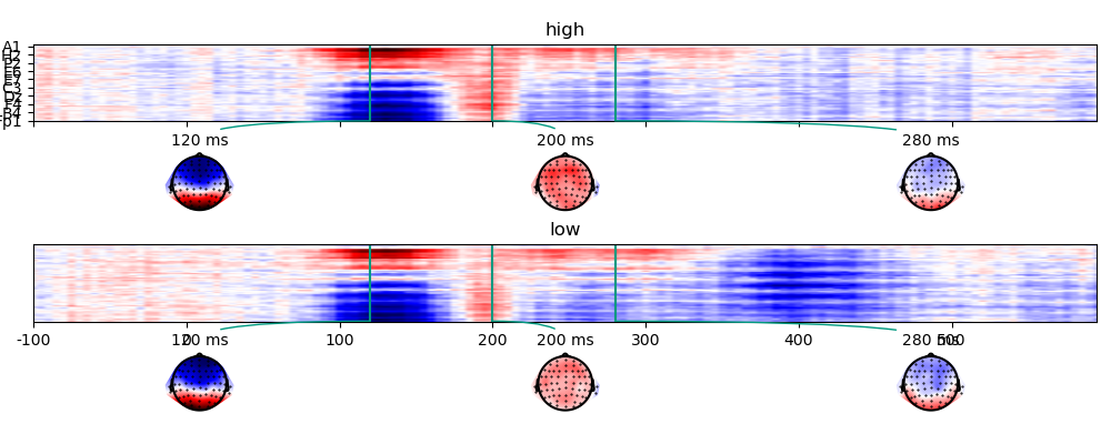
The simulated data in the two conditions:
p = plot.TopoArray('eeg', 'predictability', data=ds, columns=1, axh=2, axw=10, t=[0.120, 0.200, 0.280], head_radius=0.35)
Test between conditions
Test whether the 120 ms topography differs between the two cloze conditions. The dataset already includes one row per cell (i.e., per cloze condition and subject). Consequently, we can just index the topography at the desired time point:
topography = ds['eeg'].sub(time=0.120)
# normalize the data in accordance with McCarth & Wood (1985)
topography = normalize_in_cells(topography, 'sensor', 'predictability', ds)
# "melt" the topography NDVar to turn the sensor dimension into a Factor
ds_topography = table.melt_ndvar(topography, 'sensor', ds=ds)
# Note EEG is a single column, and the last column indicates the sensor
ds_topography.head()
ANOVA to test whether the effect of predictability differs between sensors:
test.ANOVA('eeg', 'predictability * sensor * subject', data=ds_topography)
The non-significant interaction suggests that the effect of predictability does not differ between sensors, i.e., the topographies do not differ, which is consistent with being generated by the same underlying neural sources.
Test two time points
Since we’re not interested in condition here, we first average across conditions, i.e., with the goal of having one row per subject:
ds_average = ds.aggregate('subject', drop_bad=True)
print(ds_average)
#   n    cloze     n_chars   subject
------------------------------------
0   40   0.52646   5         S00
1   40   0.51622   4.9625    S01
2   40   0.51211   5.0125    S02
3   40   0.51388   5.0375    S03
4   40   0.53115   5.05      S04
5   40   0.52163   4.9125    S05
6   40   0.53789   5.0625    S06
7   40   0.52491   4.8625    S07
8   40   0.52464   5.2125    S08
9   40   0.52559   5         S09
------------------------------------
NDVars: eeg
In order to compare two time points, we need to construct a new dataset with time point as Factor:
dss = []
for time in [0.120, 0.280]:
    ds_time = ds_average['subject',]  # A new dataset with the 'subject' variable only
    ds_time['eeg'] = ds_average['eeg'].sub(time=time)
    ds_time[:, 'time'] = f'{time * 1000:.0f} ms'
    dss.append(ds_time)
ds_times = combine(dss)
ds_times.summary()
Then, normalize the data in accordance with McCarth & Wood (1985)
topography = normalize_in_cells('eeg', 'sensor', 'time', data=ds_times)
# "melt" the topography NDVar to turn the sensor dimension into a Factor
ds_topography = table.melt_ndvar(topography, 'sensor', ds=ds_times)
# Note EEG is a single column, and the last column indicates the sensor
ds_topography.head()
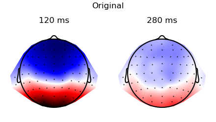
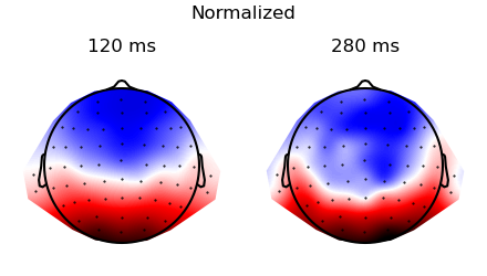
Plot the topographies before and after normalization:
p = plot.Topomap('eeg', 'time', data=ds_times, columns=2, title="Original", head_radius=0.35)
p = plot.Topomap(topography, 'time', data=ds_times, columns=2, title="Normalized", head_radius=0.35)
Compare the topographies with the ANOVA – test whether the effect of time differs between sensors:
test.ANOVA('eeg', 'time * sensor * subject', data=ds_topography)
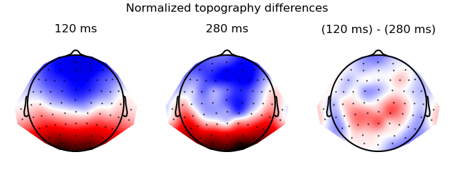
The significant interaction suggests that the effect of time differs between sensors. This means the two topographic patterns are different, suggesting that they were generated by a different constellation of underlying sources. Visualize the difference:
res = testnd.TTestRelated(topography, 'time', match='subject', data=ds_times)
p = plot.Topomap(res, columns=3, title="Normalized topography differences", head_radius=0.35)
References
Total running time of the script: (0 minutes 4.150 seconds)