Multiple regression

Multiple regression designs apply to at least two scenarios.

• Analyzing a single subject’s data when trials are associated with one or multiple continuous variables.

• Analyzing group data when subjects are associated with one or multiple individual difference variables.

Here the analysis is illustrated for a simulated dataset from a single subject. Group analysis works analogously, except that each case in the datatset would represent a different subject rather than a different trial.

For such group analysis, it is necessary to reduce each subject’s data to a single case first because multiple regression assumes a fixed effects model. Such designs are described under Two-stage test.

Simulated data

# sphinx_gallery_thumbnail_number = 2
from eelbrain import *


data = datasets.simulate_erp(snr=0.5)
data.head()

#	cloze	predictability	n_chars
0	0.026139	low	4
1	0.99529	high	5
2	0.93062	high	3
3	0.82404	high	7
4	0.17041	low	4
5	0.18508	low	4
6	0.23345	low	4
7	0.80784	high	3
8	0.24979	low	7
9	0.26753	low	4

NDVars: eeg

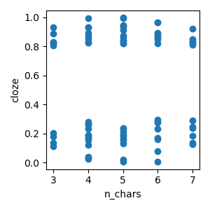
The data represents 80 trials from a simulated word reading paradigm, where each word is associated with a word length (n_chars) and predictability (cloze).

p = plot.Scatter('cloze', 'n_chars', data=data, h=3)

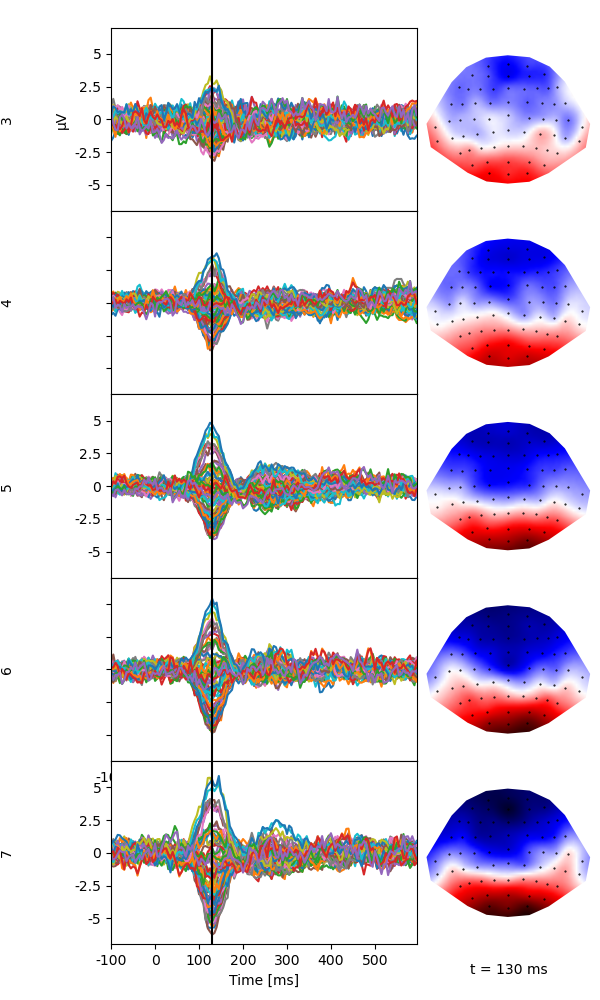
Plot the average of each level on n_chars to illustrate the linear increase of the response around 130 ms with n_char.

p = plot.TopoButterfly('eeg', 'n_chars', data=data, t=.130, axh=2, w=6)

Multiple regression

Fit a multiple regression model. Estimate $p$-values using a cluster-based permuatation test, using a cluster-forming threshold of uncorrected $p$=.05. For this example, only 500 permutations are used. When accuracy counts, it is recommended to use 10,000 permutations (the default).

lm = testnd.LM('eeg', 'n_chars + cloze', data=data, tstart=0.050, tstop=0.500, pmin=0.05, samples=500)

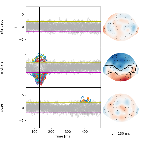
A quick plot suggests an early effect related to n_chars around 130 ms, and a later effect of cloze around 400 ms:

p = plot.TopoButterfly(lm, t=0.130, axh=2, w=6)

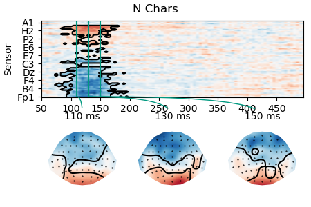
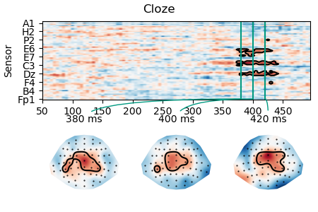
Detailed plots of the two effects show that the cluster is quite variable due to noise in the data.

p = plot.TopoArray(lm.masked_parameter_map('n_chars'), t=[0.110, 0.130, 0.150], title='N Chars')
p = plot.TopoArray(lm.masked_parameter_map('cloze'), t=[0.380, 0.400, 0.420], title='Cloze')

• 
• 

To access some of the test results we need to know the index of different effects:

lm.effects

('intercept', 'n_chars', 'cloze')

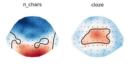
Create a plot that shows the spatial cluster extent across time.

EFFECTS = [
    ('n_chars', (0.110, 0.150)),
    ('cloze', (0.380, 0.420)),
]

t_maps = []
for effect, time in EFFECTS:
    # t-maps are retrieved by effect name
    t = lm.t(effect).mean(time=time)
    # p-maps are stored in a list, so we need to know the index of te effect
    index = lm.effects.index(effect)
    # We are interested in the maximal spatial cluster extent, i.e., any sensor that is part of the cluster at any time
    p = lm.p[index].min(time=time)
    # Create a masked average t map
    t_av = t.mask(p > 0.05)
    t_maps.append(t_av)

p = plot.Topomap(t_maps, columns=2)