ANOVA

This example performs mass-univariate ANOVA using testnd.ANOVA. The example shows a 2 x 2 repeated measures ANOVA. For specifying different ANOVA type models see the test.ANOVA documentation. The example uses simulated data meant to vaguely resemble data from an N400 experiment (not intended as a physiologically realistic simulation).

from eelbrain import *

Simulated data

Use datasets.simulate_erp() to generate a dataset simulating an N400 experiment, as in the T-test example. Set short_long=True to simulate word length as a second variable, resulting in a 2 x 2, predictability x word length design.

s_datasets = []
for subject in range(10):
    # generate data for one subject
    s_data = datasets.simulate_erp(seed=subject, short_long=True)
    # average across trials to get condition means
    s_data_agg = s_data.aggregate('predictability % length')
    # add the subject name as variable
    s_data_agg[:, 'subject'] = f'S{subject:02}'
    s_datasets.append(s_data_agg)

data = combine(s_datasets)
# Define subject as random factor (to treat it as random effect in the ANOVA)
data['subject'].random = True
data.head()

#	n	cloze	predictability	n_chars	length	subject
0	20	0.87997	high	4.6	short	S00
1	20	0.88104	high	8.2	long	S00
2	20	0.17447	low	3.6	short	S00
3	20	0.17035	low	8.9	long	S00
4	20	0.88708	high	3.8	short	S01
5	20	0.90223	high	8.4	long	S01
6	20	0.11018	low	4.3	short	S01
7	20	0.16538	low	8.25	long	S01
8	20	0.90949	high	3.95	short	S02
9	20	0.89482	high	8.25	long	S02

NDVars: eeg

Re-reference the EEG data (i.e., subtract the mean of the two mastoid channels):

data['eeg'] -= data['eeg'].mean(sensor=['M1', 'M2'])

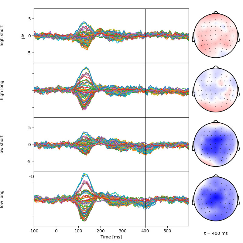
Plot the data by condition to illustrate the effect. Note 2 effects in the simulation: an early ~130 ms peak determined by word length, simulating increased visual processing for longer words; and a later “N400” predictability peak, simulated to be larger for more surprising (less predictable) words.

p = plot.TopoButterfly('eeg', 'predictability % length', t=.400, data=data, axh=2, w=8, clip='circle')

Spatio-temporal test

testnd.ANOVA provides an interface for mass-univariate ANOVA. The ANOVA function determines whether to perform a repeated measures or fixed effects ANOVA based on the model. Here, 'predictability * length * subject' is a repeated measures ANOVA because we defined data['subject'] as random effect above. Changing the model to 'predictability * length' would perform a fixed effects ANOVA.

result = testnd.ANOVA(
    'eeg',
    'predictability * length * subject',
    data=data,
    pmin=0.05,  # Use uncorrected p = 0.05 as threshold for forming clusters
    tstart=0.050,  # Find clusters in the time window from 100 ...
    tstop=0.600,  # ... to 600 ms
    samples=1000,  # smaller number of permutations to speed up the example; use 10'000 when the exact p-value matters
)

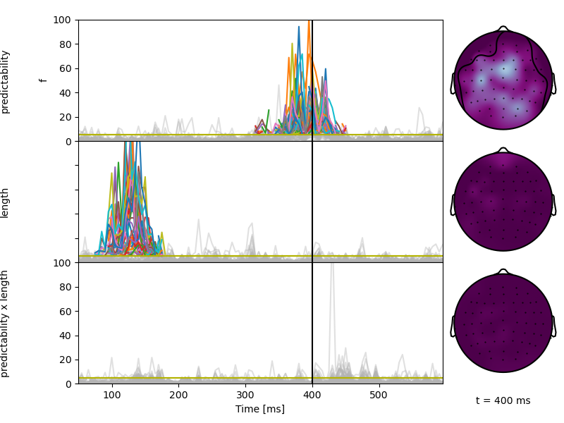
The default visualization shows F-values over time. A yellow line indicates the F-value corresponding - the pmin=0.05 parameter. In the butterfly plots, line segments that are part of a significant cluster are shown in color. In the topographic map, significant clusters are shown by outline.

p = plot.TopoButterfly(result, t=.400, axh=2, w=8, clip='circle', vmax=100)
_ = p.plot_colorbar()

• 
• 

The corresponding F-maps can be accessed on the result object:

result.f

[<NDVar 'predictability': 140 time, 65 sensor>, <NDVar 'length': 140 time, 65 sensor>, <NDVar 'predictability x length': 140 time, 65 sensor>]

Corresponding cluster statistics:

result.find_clusters(0.05)

#	id	tstart	tstop	duration	n_sensors	v	p	sig	effect
0	3	0.315	0.455	0.14	61	11800	0	***	predictability
1	2	0.075	0.185	0.11	53	12739	0	***	length