Reference
Data Classes
Primary data classes:
Dataset([items, name, caption, info, n_cases]) |
Store multiple variables pertaining to a common set of measurement cases |
Factor(x[, name, random, repeat, tile, …]) |
Container for categorial data. |
Var(x[, name, info, repeat, tile]) |
Container for scalar data. |
NDVar(x, dims, Sequence[Dimension]], name, info) |
Container for n-dimensional data. |
Datalist([items, name, fmt]) |
list subclass for including lists in in a Dataset. |
Model classes (not usually initialized by themselves but through operations on primary data-objects):
Interaction(base) |
Represents an Interaction effect. |
Model(x) |
A list of effects. |
NDVar dimensions (not usually initialized by themselves but through
load functions):
Case(n[, connectivity]) |
Case dimension |
Categorial(name, values[, connectivity]) |
Simple categorial dimension |
Scalar(name, values[, unit, tick_format, …]) |
Scalar dimension |
Sensor(locs[, names, sysname, proj2d, …]) |
Dimension class for representing sensor information |
SourceSpace(vertices[, subject, src, …]) |
MNE surface-based source space |
VolumeSourceSpace(vertices[, subject, src, …]) |
MNE volume source space |
Space(directions[, name]) |
Represent multiple directions in space |
UTS(tmin, tstep, nsamples) |
Dimension object for representing uniform time series |
File I/O
Eelbrain objects can be
pickled. Eelbrain’s own
pickle I/O functions provide backwards compatibility for Eelbrain objects
(although files saved in Python 3 can only be opened in Python 2 if they are
saved with protocol<=2):
save.pickle(obj, dest, protocol) |
Pickle a Python object. |
load.unpickle(path) |
Load pickled Python objects from a file. |
load.arrow([file_path]) |
Load object serialized with pyarrow. |
save.arrow(obj[, dest]) |
Save a Python object with pyarrow. |
load.update_subjects_dir(obj, subjects_dir) |
Update NDVar SourceSpace.subjects_dir attributes |
Import
Functions and modules for loading specific file formats as Eelbrain object:
load.wav([filename, name, backend]) |
Load a wav file as NDVar |
load.tsv(path, names, bool]=True, types, …) |
Load a Dataset from a text file. |
load.eyelink |
Tools for loading data form eyelink edf files. |
load.fiff |
Tools for importing data through mne. |
load.txt |
Tools for loading data from text files. |
load.besa |
Tools for loading data from the BESA-MN pipeline. |
Export
Dataset with only univariate data can be saved as text using the
save_txt() method. Additional export functions:
save.txt(iterator[, fmt, delim, dest]) |
Write any object that supports iteration to a text file. |
save.wav(ndvar[, filename, toint]) |
Save an NDVar as wav file |
Sorting and Reordering
align(d1, d2[, i1, i2, out]) |
Align two data-objects based on index variables |
align1(d, to[, by, out]) |
Align a data object to an index variable |
Celltable(y[, x, match, sub, cat, ds, …]) |
Divide y into cells defined by x. |
choose(choice, sources[, name]) |
Combine data-objects picking from a different object for each case |
combine(items[, name, check_dims, …]) |
Combine a list of items of the same type into one item. |
shuffled_index(n[, cells]) |
Return an index to shuffle a data-object |
NDVar Initializers
gaussian(center, width, time) |
Gaussian window NDVar |
powerlaw_noise(dims, exponent) |
Gaussian  noise. noise. |
NDVar Operations
NDVar objects support the native abs() and round()
functions. See also NDVar methods.
Butterworth(low, high, order[, sfreq]) |
Butterworth filter |
complete_source_space(ndvar[, fill, mask]) |
Fill in missing vertices on an NDVar with a partial source space |
concatenate(ndvars[, dim, name, tmin, info, …]) |
Concatenate multiple NDVars |
convolve(h, x[, ds, name]) |
Convolve h and x along the time dimension |
correlation_coefficient(x, y[, dim, name]) |
Correlation between two NDVars along a specific dimension |
cross_correlation(in1, in2[, name]) |
Cross-correlation between two NDVars along the time axis |
cwt_morlet(y, freqs[, use_fft, n_cycles, …]) |
Time frequency decomposition with Morlet wavelets (mne-python) |
dss(ndvar) |
Denoising source separation (DSS) |
filter_data(ndvar, l_freq, h_freq[, …]) |
Apply mne.filter.filter_data() to an NDVar |
find_intervals(ndvar[, interpolate]) |
Find intervals from a boolean NDVar |
find_peaks(ndvar) |
Find local maxima in an NDVar |
frequency_response(b[, frequencies]) |
Frequency response for a FIR filter |
label_operator(labels[, operation, exclude, …]) |
Convert labeled NDVar into a matrix operation to extract label values |
labels_from_clusters(clusters[, names]) |
Create Labels from source space clusters |
maximum(ndvars, name) |
Element-wise maximum of multiple NDVar objects |
minimum(ndvars, name) |
Element-wise minimum of multiple NDVar objects |
morph_source_space(ndvar[, subject_to, …]) |
Morph source estimate to a different MRI subject |
neighbor_correlation(x[, dim, obs, name]) |
Calculate Neighbor correlation |
psd_welch(ndvar[, fmin, fmax, n_fft, …]) |
Power spectral density with Welch’s method |
resample(ndvar, sfreq[, npad, window, pad, name]) |
Resample an NDVar along the time dimension |
segment(continuous, times, tstart, tstop[, …]) |
Segment a continuous NDVar |
set_parc(ndvar, parc[, dim]) |
Change the parcellation of an NDVar with SourceSpace dimension |
set_time(ndvar, time, …) |
Crop and/or pad an NDVar to match the time axis time |
set_tmin(ndvar[, tmin]) |
Shift the time axis of an NDVar relative to its data |
xhemi(ndvar[, mask, hemi, parc]) |
Project data from both hemispheres to hemi of fsaverage_sym |
Reverse Correlation
boosting(y, x, tstart, tstop[, scale_data, …]) |
Estimate a linear filter with coordinate descent |
BoostingResult(y, x, tstart, tstop, …[, …]) |
Result from boosting a temporal response function |
epoch_impulse_predictor(shape[, value, …]) |
Time series with one impulse for each of n epochs |
Tables
Manipulate data tables and compile information about data objects such as cell frequencies:
table.cast_to_ndvar(data, dim_values, match) |
Create an NDVar by converting a data column to a dimension |
table.difference(y, x, c1, c0, match[, sub, …]) |
Subtract data in one cell from another |
table.frequencies(y[, x, of, sub, ds]) |
Calculate frequency of occurrence of the categories in y |
table.melt(name, cells, cell_var_name, ds[, …]) |
Restructure a Dataset such that a measured variable is in a single column |
table.melt_ndvar(ndvar[, dim, cells, ds, …]) |
Transform data to long format by converting an NDVar dimension into a variable |
table.repmeas(y, x, match[, sub, ds]) |
Create a repeated-measures table |
table.stats(y, row[, col, match, sub, fmt, …]) |
Make a table with statistics |
Statistics
Univariate statistical tests:
test.Correlation(y, …) |
Pearson product moment correlation between y and x |
test.TTest1Sample(y, str], match, …) |
1-sample t-test |
test.TTestInd(y, str], x, …) |
Independent measures t-test |
test.TTestRel(y, str], x, …) |
Related-measures t-test |
test.anova(y, x[, sub, ds, title, caption]) |
Univariate ANOVA |
test.pairwise(y, str], x, …) |
Pairwise comparison table |
test.ttest(y[, x, against, match, sub, …]) |
T-tests for one or more samples |
test.correlations(y, x[, cat, sub, ds, asds]) |
Correlation with one or more predictors |
test.pairwise_correlations(xs[, sub, ds, labels]) |
Pairwise correlation table |
test.MannWhitneyU(y, str], x, …) |
Mann-Whitney U-test (non-parametric independent measures test) |
test.WilcoxonSignedRank(y, str], x, …) |
Wilcoxon signed-rank test (non-parametric related measures test) |
test.lilliefors(data[, formatted]) |
Lilliefors’ test for normal distribution |
Mass-Univariate Statistics
testnd.ttest_1samp(y, str], popmean, match, …) |
Mass-univariate one sample t-test |
testnd.ttest_rel(y, str], x, …) |
Mass-univariate related samples t-test |
testnd.ttest_ind(y, str], x, …) |
Mass-univariate independent samples t-test |
testnd.t_contrast_rel(y, str], x, …) |
Mass-univariate contrast based on t-values |
testnd.anova(y, str], x, …) |
Mass-univariate ANOVA |
testnd.corr(y, str], x, str], norm, …) |
Mass-univariate correlation |
testnd.Vector(y, str], match, …) |
Test a vector field for vectors with non-random direction |
testnd.VectorDifferenceRelated(y, str], x, …) |
Test difference between two vector fields for non-random direction |
By default the tests in this module produce maps of statistical parameters along with maps of p-values uncorrected for multiple comparison. Using different parameters, different methods for multiple comparison correction can be applied (for more details and options see the documentation for individual tests):
- 1: permutation for maximum statistic (
samples=n) - Look for the maximum
value of the test statistic in
npermutations and calculate a p-value for each data point based on this distribution of maximum statistics. - 2: Threshold-based clusters (
samples=n, pmin=p) - Find clusters of data
points where the original statistic exceeds a value corresponding to an
uncorrected p-value of
p. For each cluster, calculate the sum of the statistic values that are part of the cluster. Do the same innpermutations of the original data and retain for each permutation the value of the largest cluster. Evaluate all cluster values in the original data against the distributiom of maximum cluster values (see [1]). - 3: Threshold-free cluster enhancement (
samples=n, tfce=True) - Similar to (1), but each statistical parameter map is first processed with the cluster-enhancement algorithm (see [2]). This is the most computationally intensive option.
Two-stage tests
Two-stage tests proceed by estimating parameters for a fixed effects model for
each subject, and then testing hypotheses on these parameter estimates on the
group level. Two-stage tests are implemented by fitting an LM
for each subject, and then combining them in a LMGroup to
retrieve coefficients for group level statistics (see recipe for
recipe-regression).
testnd.LM(y, model[, ds, coding, subject, sub]) |
Fixed effects linear model |
testnd.LMGroup(lms) |
Group level analysis for linear model LM objects |
References
| [1] | Maris, E., & Oostenveld, R. (2007). Nonparametric statistical testing of EEG- and MEG-data. Journal of Neuroscience Methods, 164(1), 177-190. 10.1016/j.jneumeth.2007.03.024 |
| [2] | Smith, S. M., and Nichols, T. E. (2009). Threshold-Free Cluster Enhancement: Addressing Problems of Smoothing, Threshold Dependence and Localisation in Cluster Inference. NeuroImage, 44(1), 83-98. 10.1016/j.neuroimage.2008.03.061 |
Plotting
Plot univariate data (Var objects):
plot.Barplot(y[, x, match, sub, cells, …]) |
Barplot for a continuous variable |
plot.BarplotHorizontal(y[, x, match, sub, …]) |
Horizontal barplot for a continuous variable |
plot.Boxplot(y[, x, match, sub, cells, …]) |
Boxplot for a continuous variable |
plot.PairwiseLegend([size, trend]) |
Legend for colors used in pairwise comparisons |
plot.Correlation(y, x[, cat, sub, ds, c, …]) |
Plot the correlation between two variables |
plot.Histogram(y[, x, match, sub, ds, …]) |
Histogram plots with tests of normality |
plot.Regression(y, x[, cat, match, sub, ds, …]) |
Plot the regression of y on x |
plot.Timeplot(y, categories, time[, match, …]) |
Plot a variable over time |
Color tools for plotting:
plot.colors_for_categorial(x[, hue_start, cmap]) |
Automatically select colors for a categorial model |
plot.colors_for_oneway(cells[, hue_start, …]) |
Define colors for a single factor design |
plot.colors_for_twoway(x1_cells, x2_cells[, …]) |
Define cell colors for a two-way design |
plot.soft_threshold_colormap(cmap, …[, …]) |
Soft-threshold a colormap to make small values transparent |
plot.two_step_colormap(left_max, left[, …]) |
Colormap using lightness to extend range |
plot.ColorBar(cmap[, vmin, vmax, label, …]) |
A color-bar for a matplotlib color-map |
plot.ColorGrid(row_cells, column_cells, colors) |
Plot colors for a two-way design in a grid |
plot.ColorList(colors[, cells, labels, size, h]) |
Plot colors with labels |
Plot uniform time-series:
plot.LineStack(y[, x, sub, ds, offset, …]) |
Stack multiple lines vertically |
plot.UTS(y[, xax, axtitle, ds, sub, xlabel, …]) |
Value by time plot for UTS data |
plot.UTSClusters(res[, pmax, ptrend, …]) |
Plot permutation cluster test results |
plot.UTSStat(y[, x, xax, match, sub, ds, …]) |
Plot statistics for a one-dimensional NDVar |
Plot multidimensional uniform time series:
plot.Array(y[, xax, xlabel, ylabel, …]) |
Plot UTS data to a rectangular grid. |
plot.Butterfly(y[, xax, sensors, axtitle, …]) |
Butterfly plot for NDVars |
Plot topographic maps of sensor space data:
plot.TopoArray(y[, xax, ds, sub, vmax, …]) |
Channel by sample plots with topomaps for individual time points |
plot.TopoButterfly(y[, xax, ds, sub, vmax, …]) |
Butterfly plot with corresponding topomaps |
plot.Topomap(y[, xax, ds, sub, vmax, vmin, …]) |
Plot individual topogeraphies |
plot.TopomapBins(y[, xax, ds, sub, …]) |
Topomaps in time-bins |
Plot sensor layout maps:
plot.SensorMap(sensors[, labels, proj, …]) |
Plot sensor positions in 2 dimensions |
plot.SensorMaps(sensors[, select, proj, …]) |
Multiple views on a sensor layout. |
xax parameter
Many plots have an xax parameter which is used to sort the data in y
into different categories and plot them on separate axes. xax can be
specified through categorial data, or as a dimension in y.
If a categorial data object is specified for xax, y is split into the
categories in xax, and for every cell in xax a separate subplot is
shown. For example, while
>>> plot.Butterfly('meg', ds=ds)
will create a single Butterfly plot of the average response,
>>> plot.Butterfly('meg', 'subject', ds=ds)
where 'subject' is the xax parameter, will create a separate subplot
for every subject with its average response.
A dimension on y can be specified through a string starting with ..
For example, to plot each case of meg separately, use:
>>> plot.Butterfly('meg', '.case', ds=ds)
General layout parameters
Most plots that also share certain layout keyword arguments. By default, all those parameters are determined automatically, but individual values can be specified manually by supplying them as keyword arguments.
h,w: scalar- Height and width of the figure. Use a number ≤ 0 to defined the size relative
to the screen (e.g.,
w=0to use the full screen width). axh,axw: scalar- Height and width of the axes.
nrow,ncol:None|int- Limit number of rows/columns. If neither is specified, a square layout is produced
margins:dictAbsolute subplot parameters (in inches). Implies
tight=False. Ifmarginsis specified,axwandaxhare interpreted exclusive of the margins, i.e.,axh=2, margins={'top': .5}for a plot with one axes will result in a total height of 2.5. Example:margins={ 'top': 0.5, # from top of figure to top axes 'bottom': 1, # from bottom of figure to bottom axes 'hspace': 0.1, # height of space between axes 'left': 0.5, # from left of figure to left-most axes 'right': 0.1, # from right of figure to right-most axes 'wspace': 0.1, # width of space between axes }
ax_aspect: scalar- Width / height aspect of the axes.
frame:bool|strHow to frame the axes of the plot. Options:
True(default): normal matplotlib frame, spines around axesFalse: omit top and right spines't': draw spines at x=0 and y=0, common for ERPs'none': no spines at all
name:str- Window title (not displayed on the figure itself).
title:str- Figure title (displayed on the figure).
tight:bool- Use matplotlib’s
tight_layoutto resize all axes to fill the figure. right_of: eelbrain plot- Position the new figure to the right of this figure.
Plots that do take those parameters can be identified by the **layout in
their function signature.
GUI Interaction
By default, new plots are automatically shown and, if the Python interpreter is in interactive mode the GUI main loop is started. This behavior can be controlled with 2 arguments when constructing a plot:
- show : bool
- Show the figure in the GUI (default True). Use False for creating figures and saving them without displaying them on the screen.
- run : bool
- Run the Eelbrain GUI app (default is True for interactive plotting and False in scripts).
The behavior can also be changed globally using configure().
By default, Eelbrain plots open in windows with enhance GUI features such as
copying a figure to the OS clip-board. To plot figures in bare matplotlib
windows, configure() Eelbrain with eelbrain.configure(frame=False).
Plotting Brains
The plot.brain module contains specialized functions to plot
NDVar objects containing source space data.
For this it uses a subclass of PySurfer’s surfer.Brain class.
The functions below allow quick plotting.
More specific control over the plots can be achieved through the
Brain object that is returned.
plot.brain.brain(src[, cmap, vmin, vmax, …]) |
Create a Brain object with a data layer |
plot.brain.butterfly(y[, cmap, vmin, vmax, …]) |
Shortcut for a Butterfly-plot with a time-linked brain plot |
plot.brain.cluster(cluster[, vmax]) |
Plot a spatio-temporal cluster |
plot.brain.dspm(src[, fmin, fmax, fmid]) |
Plot a source estimate with coloring for dSPM values (bipolar). |
plot.brain.p_map(p_map[, param_map, p0, p1, …]) |
Plot a map of p-values in source space. |
plot.brain.annot(annot[, subject, surf, …]) |
Plot the parcellation in an annotation file |
plot.brain.annot_legend(lh, rh, *args, **kwargs) |
Plot a legend for a freesurfer parcellation |
Brain(subject, hemi[, surf, title, cortex, …]) |
PySurfer Brain subclass returned by plot.brain functions |
plot.brain.SequencePlotter() |
Grid of anatomical images in one figure |
plot.GlassBrain(ndvar[, cmap, vmin, vmax, …]) |
Plot 2d projections of a brain volume |
plot.GlassBrain.butterfly(y[, cmap, vmin, …]) |
Shortcut for a butterfly-plot with a time-linked glassbrain plot |
In order to make custom plots, a Brain figure
without any data added can be created with
plot.brain.brain(ndvar.source, mask=False).
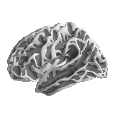
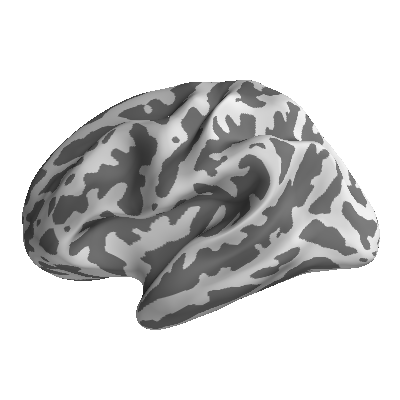
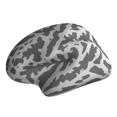
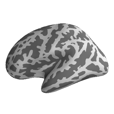
Surface options for plotting data on fsaverage:
white
|
smoothwm
|
inflated_pre
|
inflated
|
inflated_avg
|
sphere
|

GUIs
Tools with a graphical user interface (GUI):
gui.select_components(path, ds[, sysname, …]) |
GUI for selecting ICA-components |
gui.select_epochs(ds[, data, accept, blink, …]) |
GUI for rejecting trials of MEG/EEG data |
gui.load_stcs() |
GUI for detecting and loading source estimates |
Controlling the GUI Application
Eelbrain uses a wxPython based application to create GUIs. This GUI appears as a separate application with its own Dock icon. The way that control of this GUI is managed depends on the environment form which it is invoked.
When Eelbrain plots are created from within iPython, the GUI is managed in the
background and control returns immediately to the terminal. There might be cases
in which this is not desired, for example when running scripts. After execution
of a script finishes, the interpreter is terminated and all associated plots are
closed. To avoid this, the command gui.run(block=True) can be inserted at
the end of the script, which will keep all gui elements open until the user
quits the GUI application (see gui.run() below).
In interpreters other than iPython, input can not be processed from the GUI
and the interpreter shell at the same time. In that case, the GUI application
is activated by default whenever a GUI is created in interactive mode
(this can be avoided by passing run=False to any plotting function).
While the application is processing user input,
the shell can not be used. In order to return to the shell, quit the
application (the python/Quit Eelbrain menu command or Command-Q). In order to
return to the terminal without closing all windows, use the alternative
Go/Yield to Terminal command (Command-Alt-Q). To return to the application
from the shell, run gui.run(). Beware that if you terminate the Python
session from the terminal, the application is not given a chance to assure that
information in open windows is saved.
gui.run([block]) |
Hand over command to the GUI (quit the GUI to return to the terminal) |
Formatted Text
The fmtxt submodule provides tools for exporting results. Most eelbrain
functions and methods that print tables in fact return fmtxt objects,
which can be exported in different formats, for example:
>>> ds = datasets.get_uv()
>>> type(ds.head())
eelbrain.fmtxt.Table
This means that the result can be exported as formatted text, for example:
>>> fmtxt.save_pdf(ds.head())
Available export methods:
fmtxt.copy_pdf(fmtext) |
Copy an FMText object to the clipboard as PDF. |
fmtxt.copy_tex(fmtext) |
Copy an FMText object to the clipboard as tex code |
fmtxt.save_html(fmtext[, path, …]) |
Save an FMText object in HTML format |
fmtxt.save_pdf(fmtext[, path]) |
Save an FMText object as a pdf (requires LaTeX installation) |
fmtxt.save_rtf(fmtext[, path]) |
Save an FMText object in Rich Text format |
fmtxt.save_tex(fmtext[, path]) |
Save an FMText object as TeX code |
MNE-Experiment
The MneExperiment class serves as a base class for analyzing MEG
data (gradiometer only) with MNE:
MneExperiment([root, find_subjects]) |
Analyze an MEG experiment (gradiometer only) with MNE |
ROITestResult(subjects, samples, …) |
Test results for temporal tests in one or more ROIs |
ROI2StageResult(subjects, samples, …) |
Test results for 2-stage tests in one or more ROIs |
See also
For the guide on working with the MneExperiment class see The MneExperiment Pipeline.
Datasets
Datasets for experimenting and testing:
datasets.get_loftus_masson_1994() |
Dataset used for illustration purposes by Loftus and Masson (1994) |
datasets.get_mne_sample([tmin, tmax, …]) |
Load events and epochs from the MNE sample data |
datasets.get_uts([utsnd, seed, nrm, vector3d]) |
Create a sample Dataset with 60 cases and random data. |
datasets.get_uv([seed, nrm, vector]) |
Dataset with random univariate data |
datasets.simulate_erp([n_trials, seed]) |
Simulate event-related EEG data |
Configuration
-
eelbrain.configure(n_workers=None, frame=None, autorun=None, show=None, format=None, figure_background=None, prompt_toolkit=None, animate=None, nice=None, tqdm=None)¶ Set basic configuration parameters for the current session
Parameters: - n_workers : bool | int
Number of worker processes to use in multiprocessing enabled computations.
Falseto disable multiprocessing.True(default) to use as many processes as cores are available. Negative numbers to use all but n available CPUs.- frame : bool
Open figures in the Eelbrain application. This provides additional functionality such as copying a figure to the clipboard. If False, open figures as normal matplotlib figures.
- autorun : bool
When a figure is created, automatically enter the GUI mainloop. By default, this is True when the figure is created in interactive mode but False when the figure is created in a script (in order to run the GUI at a specific point in a script, call
eelbrain.gui.run()).- show : bool
Show plots on the screen when they’re created (disable this to create plots and save them without showing them on the screen).
- format : str
Default format for plots (for example “png”, “svg”, …).
- figure_background : bool | matplotlib color
While
matplotlibuses a gray figure background by default, Eelbrain uses white. Set this parameter toFalseto use the default frommatplotlib.rcParams, or set it to a valid matplotblib color value to use an arbitrary color.Trueto revert to the default white.- prompt_toolkit : bool
In IPython 5, prompt_toolkit allows running the GUI main loop in parallel to the Terminal, meaning that the IPython terminal and GUI windows can be used without explicitly switching between Terminal and GUI. This feature is enabled by default, but can be disabled by setting
prompt_toolkit=False.- animate : bool
Animate plot navigation (default True).
- nice : int [-20, 19]
Scheduling priority for muliprocessing (larger number yields more to other processes; negative numbers require root privileges).
- tqdm : bool
Enable or disable
tqdmprogress bars.