Note
Click here to download the full example code
ANCOVA
Example 1
Based on [1], Exercises (page 8).
Show the model
Out:
intercept   Hours   Genotype                 Hours x Genotype
-----------------------------------------------------------------------------
1           8       1    0    0    0    0    8      0      0      0      0
1           12      1    0    0    0    0    12     0      0      0      0
1           16      1    0    0    0    0    16     0      0      0      0
1           24      1    0    0    0    0    24     0      0      0      0
1           8       0    1    0    0    0    0      8      0      0      0
1           12      0    1    0    0    0    0      12     0      0      0
1           16      0    1    0    0    0    0      16     0      0      0
1           24      0    1    0    0    0    0      24     0      0      0
1           8       0    0    1    0    0    0      0      8      0      0
1           12      0    0    1    0    0    0      0      12     0      0
1           16      0    0    1    0    0    0      0      16     0      0
1           24      0    0    1    0    0    0      0      24     0      0
1           8       0    0    0    1    0    0      0      0      8      0
1           12      0    0    0    1    0    0      0      0      12     0
1           16      0    0    0    1    0    0      0      0      16     0
1           24      0    0    0    1    0    0      0      0      24     0
1           8       0    0    0    0    1    0      0      0      0      8
1           12      0    0    0    0    1    0      0      0      0      12
1           16      0    0    0    0    1    0      0      0      0      16
1           24      0    0    0    0    1    0      0      0      0      24
1           8       0    0    0    0    0    0      0      0      0      0
1           12      0    0    0    0    0    0      0      0      0      0
1           16      0    0    0    0    0    0      0      0      0      0
1           24      0    0    0    0    0    0      0      0      0      0
ANCOVA
Out:
ANOVA

                      SS   df     MS          F        p
--------------------------------------------------------
Hours               7.06    1   7.06   54.90***   < .001
Genotype           27.88    5   5.58   43.36***   < .001
Hours x Genotype    3.15    5   0.63    4.90*       .011
Residuals           1.54   12   0.13
--------------------------------------------------------
Total              39.62   23
Plot the slopes
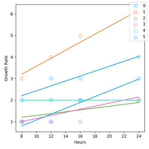
Out:
<Regression: Growth Rate ~ Hours | Genotype>
Example 2
Based on [2] (p. 118-20)
Full model, with interaction
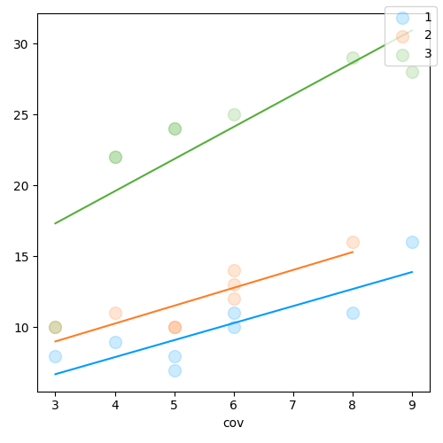
Out:
                 SS   df       MS          F        p
-----------------------------------------------------
cov          199.54    1   199.54   32.93***   < .001
A            807.82    2   403.91   66.66***   < .001
cov x A       19.39    2     9.70    1.60        .229
Residuals    109.07   18     6.06
-----------------------------------------------------
Total       1112.00   23

<Regression: None ~ cov | A>
Drop interaction term
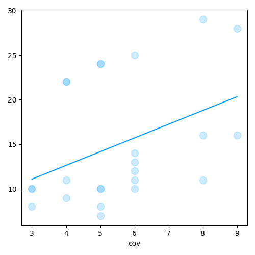
Out:
                 SS   df       MS          F        p
-----------------------------------------------------
A            807.82    2   403.91   62.88***   < .001
cov          199.54    1   199.54   31.07***   < .001
Residuals    128.46   20     6.42
-----------------------------------------------------
Total       1112.00   23

<Regression: None ~ cov>
ANCOVA with multiple covariates
Based on [3], p. 139.
Out:
id                    education   income   women   prestige   census   type
---------------------------------------------------------------------------
GOV.ADMINISTRATORS    13.11       12351    11.16   68.8       1113     prof
GENERAL.MANAGERS      12.26       25879    4.02    69.1       1130     prof
ACCOUNTANTS           12.77       9271     15.7    63.4       1171     prof
PURCHASING.OFFICERS   11.42       8865     9.11    56.8       1175     prof
CHEMISTS              14.62       8403     11.68   73.5       2111     prof
PHYSICISTS            15.64       11030    5.13    77.6       2113     prof
BIOLOGISTS            15.09       8258     25.65   72.6       2133     prof
ARCHITECTS            15.44       14163    2.69    78.1       2141     prof
CIVIL.ENGINEERS       14.52       11377    1.03    73.1       2143     prof
MINING.ENGINEERS      14.64       11023    0.94    68.8       2153     prof
# Variable summary
print(ds.summary())
Out:
Key         Type     Values
-------------------------------------------------------------------------------------------------
id          Factor   ACCOUNTANTS, AIRCRAFT.REPAIRMEN, AIRCRAFT.WORKERS, ARCHITECTS... (102 cells)
education   Var      6.38 - 15.97
income      Var      611 - 25879
women       Var      0 - 97.51
prestige    Var      14.8 - 87.2
census      Var      1113 - 9517
type        Factor   NA:4, bc:44, prof:31, wc:23
-------------------------------------------------------------------------------------------------
Fox_Prestige_data.txt: 102 cases
Out:
                         SS   df        MS          F        p
--------------------------------------------------------------
income              1131.90    1   1131.90   28.35***   < .001
education           1067.98    1   1067.98   26.75***   < .001
type                 591.16    2    295.58    7.40**      .001
income x type        951.77    2    475.89   11.92***   < .001
education x type     238.40    2    119.20    2.99        .056
Residuals           3552.86   89     39.92
--------------------------------------------------------------
Total              28346.88   97