Note
Click here to download the full example code
Cluster-based permutation t-test
This example show a cluster-based permutation test for a simple design (two conditions). The example uses simulated data meant to vaguely resemble data from an N400 experiment (not intended as a physiologically realistic simulation).
# sphinx_gallery_thumbnail_number = 3
from eelbrain import *
Simulated data
Each function call to datasets.simulate_erp() generates a dataset
equivalent to an N400 experiment for one subject.
The seed argument determines the random noise that is added to the data.
ds = datasets.simulate_erp(seed=0)
print(ds.summary())
Out:
Key         Type     Values
--------------------------------------------------------------------
eeg         NDVar    140 time, 65 sensor; -1.42723e-05 - 1.57388e-05
cloze       Var      0.00563694 - 0.997675
cloze_cat   Factor   high:40, low:40
n_chars     Var      0.314981 - 7.32121
--------------------------------------------------------------------
Dataset: 80 cases
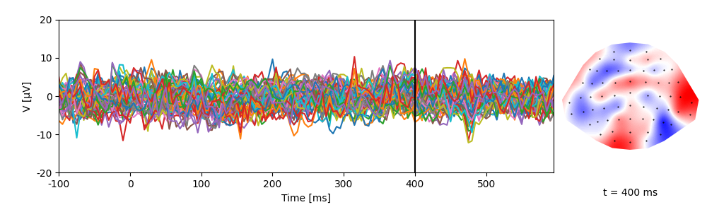
A singe trial of data:
p = plot.TopoButterfly('eeg[0]', ds=ds)
p.set_time(0.400)
The Dataset.aggregate() method computes condition averages when sorting
the data into conditions of interest. In our case, the cloze_cat variable
specified conditions 'high' and 'low' cloze:
print(ds.aggregate('cloze_cat'))
Out:
n    cloze     cloze_cat   n_chars
----------------------------------
40   0.88051   high        4.1348
40   0.17241   low         3.7869
----------------------------------
NDVars: eeg
Group level data
This loop simulates a multi-subject experiment.
It generates data and collects condition averages for 10 virtual subjects.
For group level analysis, the collected data are combined in a Dataset:
dss = []
for subject in range(10):
    # generate data for one subject
    ds = datasets.simulate_erp(seed=subject)
    # average across trials to get condition means
    ds_agg = ds.aggregate('cloze_cat')
    # add the subject name as variable
    ds_agg[:, 'subject'] = f'S{subject:02}'
    dss.append(ds_agg)

ds = combine(dss)
# make subject a random factor (to treat it as random effect for ANOVA)
ds['subject'].random = True
print(ds.head())
Out:
n    cloze     cloze_cat   n_chars   subject
--------------------------------------------
40   0.88051   high        4.1348    S00
40   0.17241   low         3.7869    S00
40   0.89466   high        3.9876    S01
40   0.13778   low         4.5732    S01
40   0.90215   high        4.2181    S02
40   0.12206   low         3.9199    S02
40   0.88503   high        3.9107    S03
40   0.14273   low         4.2281    S03
40   0.90499   high        4.0993    S04
40   0.15732   low         3.4625    S04
--------------------------------------------
NDVars: eeg
Re-reference the EEG data (i.e., subtract the mean of the two mastoid channels):
Spatio-temporal cluster based test
Cluster-based tests are based on identifying clusters of meaningful effects, i.e.,
groups of adjacent sensors that show the same effect (see testnd for references).
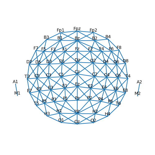
In order to find clusters, the algorithm needs to know which channels are
neighbors. This information is refered to as the sensor connectivity (i.e., which sensors
are connected). The connectivity graph can be visualized to confirm that it is set correctly.
p = plot.SensorMap(ds['eeg'], connectivity=True)
With the correct connectivity, we can now compute a cluster-based permutation test for a related measures t-test:
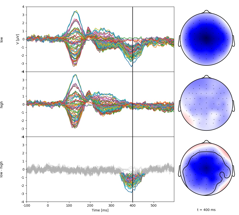
Plot the test result. The top two rows show the two condition averages. The bottom butterfly plot shows the difference with only significant regions in color. The corresponding topomap shows the topography at the marked time point, with the significant region circled (in an interactive environment, the mouse can be used to update the time point shown).
p = plot.TopoButterfly(res, clip='circle')
p.set_time(0.400)
Generate a table with all significant clusters:
Out:
id   tstart   tstop   duration   n_sensors   v         p            sig
-----------------------------------------------------------------------
42   0.34     0.465   0.125      61          -5026.8   0.00097752   ***
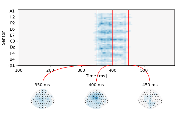
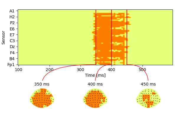
Retrieve the cluster map using its ID and visualize the spatio-temporal extent of the cluster:
cluster_id = clusters[0, 'id']
cluster = res.cluster(cluster_id)
p = plot.TopoArray(cluster, interpolation='nearest')
p.set_topo_ts(.350, 0.400, 0.450)
Often it is desirable to summarize values in a cluster. This is especially useful in more complex designs. For example, after finding a signficant interaction effect in an ANOVA, one might want to follow up with a pairwise test of the value in the cluster. This can often be achieved using binary masks based on the cluster. Using the cluster identified above, generate a binary mask:
mask = cluster != 0
p = plot.TopoArray(mask, cmap='Wistia')
p.set_topo_ts(.350, 0.400, 0.450)
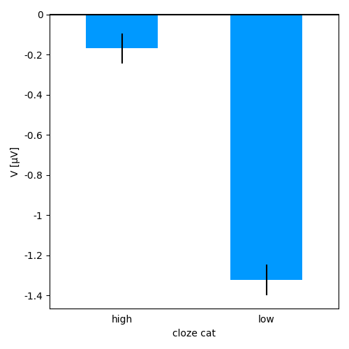
Such a spatio-temporal boolean mask can be used
to extract the value in the cluster for each condition/participant.
Since mask contains both time and sensor dimensions, using it with
the NDVar.mean() method collapses across these dimensions and
returns a scalar for each case (i.e., for each condition/subject).
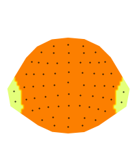
Similarly, a mask consisting of a cluster of sensors can be used to
visualize the time course in that region of interest. A straight forward
choice is to use all sensors that were part of the cluster (mask)
at any point in time:
roi = mask.any('time')
p = plot.Topomap(roi, cmap='Wistia')
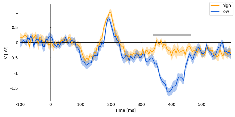
When using a mask that ony contains a sensor dimension (roi),
NDVar.mean() collapses across sensors and returns a value for each time
point, i.e. the time course in sensors involved in the cluster:
ds['cluster_timecourse'] = ds['eeg'].mean(roi)
p = plot.UTSStat('cluster_timecourse', 'cloze_cat', match='subject', ds=ds, frame='t')
# mark the duration of the spatio-temporal cluster
p.set_clusters(clusters, y=0.25e-6)
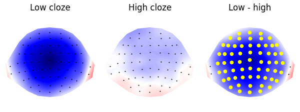
Now visualize the cluster topography, marking significant sensors:
time_window = (clusters[0, 'tstart'], clusters[0, 'tstop'])
c1_topo = res.c1_mean.mean(time=time_window)
c0_topo = res.c0_mean.mean(time=time_window)
diff_topo = res.difference.mean(time=time_window)
p = plot.Topomap([c1_topo, c0_topo, diff_topo], axtitle=['Low cloze', 'High cloze', 'Low - high'], ncol=3)
p.mark_sensors(roi, -1)
Temporal cluster based test
Alternatively, if a spatial region of interest exists, a univariate time
course can be extracted and submitted to a temporal cluster based test. For
example, the N400 is typically expected to be strong at sensor Cz:
ds['eeg_cz'] = ds['eeg'].sub(sensor='Cz')
res_timecoure = testnd.ttest_rel(
    'eeg_cz', 'cloze_cat', 'low', 'high', match='subject', ds=ds,
    pmin=0.05,  # Use uncorrected p = 0.05 as threshold for forming clusters
    tstart=0.100,  # Find clusters in the time window from 100 ...
    tstop=0.600,  # ... to 600 ms
)
clusters = res_timecoure.find_clusters(0.05)
print(clusters)

p = plot.UTSStat('eeg_cz', 'cloze_cat', match='subject', ds=ds, frame='t')
p.set_clusters(clusters, y=0.25e-6)
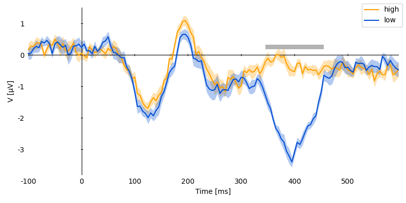
Out:
id   tstart   tstop   duration   v        p   sig
-------------------------------------------------
5    0.345    0.455   0.11       -192.1   0   ***
Total running time of the script: ( 0 minutes 9.386 seconds)