Note

Click here to download the full example code

Introduction¶

Data are represented with there primary data-objects:

Factor for categorial variables
Var for scalar variables
NDVar for multidimensional data (e.g. a variable measured at different time points)

Multiple variables belonging to the same dataset can be grouped in a Dataset object.

Factor¶

A Factor is a container for one-dimensional, categorial data: Each case is described by a string label. The most obvious way to initialize a Factor is a list of strings:

# sphinx_gallery_thumbnail_number = 5
from eelbrain import *

a = Factor(['a', 'a', 'a', 'a', 'b', 'b', 'b', 'b'], name='A')
print(a)

Out:

Factor(['a', 'a', 'a', 'a', 'b', 'b', 'b', 'b'], name='A')

Since Factor initialization simply iterates over the given data, the same Factor could be initialized with:

a = Factor('aaaabbbb', name='A')
print(a)

Out:

Factor(['a', 'a', 'a', 'a', 'b', 'b', 'b', 'b'], name='A')

There are other shortcuts to initialize factors (see also the Factor class documentation):

a = Factor(['a', 'b', 'c'], repeat=4, name='A')
print(a)

Out:

Factor(['a', 'a', 'a', 'a', 'b', 'b', 'b', 'b', 'c', 'c', 'c', 'c'], name='A')

Indexing works like for arrays:

print(a[0])
print(a[0:6])

Out:

a
Factor(['a', 'a', 'a', 'a', 'b', 'b'], name='A')

All values present in a Factor are accessible in its Factor.cells attribute:

print(a.cells)

Out:

('a', 'b', 'c')

Based on the Factor’s cell values, boolean indexes can be generated:

print(a == 'a')
print(a.isany('a', 'b'))
print(a.isnot('a', 'b'))

Out:

[ True  True  True  True False False False False False False False False]
[ True  True  True  True  True  True  True  True False False False False]
[False False False False False False False False  True  True  True  True]

Interaction effects can be constructed from multiple factors with the % operator:

b = Factor(['d', 'e'], repeat=2, tile=3, name='B')
print(b)
i = a % b
print(i)

Out:

Factor(['d', 'd', 'e', 'e', 'd', 'd', 'e', 'e', 'd', 'd', 'e', 'e'], name='B')
A % B

Interaction effects are in many ways interchangeable with factors in places where a categorial model is required:

print(i.cells)
print(i == ('a', 'd'))

Out:

(('a', 'd'), ('a', 'e'), ('b', 'd'), ('b', 'e'), ('c', 'd'), ('c', 'e'))
[ True  True False False False False False False False False False False]

Var¶

The Var class is a container for one-dimensional numpy.ndarray:

y = Var([1, 2, 3, 4, 5, 6])
print(y)

Out:

Var([1, 2, 3, 4, 5, 6])

Indexing works as for factors

print(y[5])
print(y[2:])

Out:

6
Var([3, 4, 5, 6])

Many array operations can be performed on the object directly

print(y + 1)

Out:

Var([2, 3, 4, 5, 6, 7])

For any more complex operations the corresponding numpy.ndarray can be retrieved in the Var.x attribute:

print(y.x)

Out:

[1 2 3 4 5 6]

Note

The Var.x attribute is not intended to be replaced; rather, a new Var object should be created for a new array.

NDVar¶

NDVar objects are containers for multidimensional data, and manage the description of the dimensions along with the data. NDVar objects are often not constructed from scratch but imported from existing data. For example, mne source estimates can be imported with load.fiff.stc_ndvar(). As an example, consider data from a simulated EEG experiment:

ds = datasets.simulate_erp()
eeg = ds['eeg']
print(eeg)

Out:

<NDVar 'eeg': 80 case, 140 time, 65 sensor>

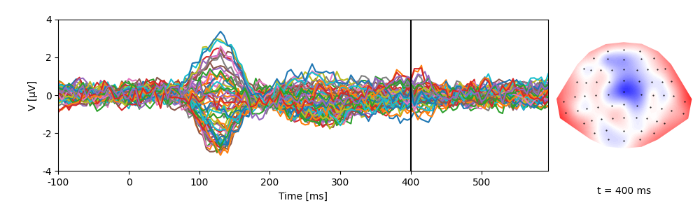
This representation shows that eeg contains 80 trials of data (cases), with 140 time points and 35 EEG sensors. Since eeg contains information on the dimensions like sensor locations, plotting functions can take advantage of that:

p = plot.TopoButterfly(eeg)
p.set_time(0.400)

NDVar offer functionality similar to numpy.ndarray, but take into account the properties of the dimensions. For example, through the NDVar.sub() method, indexing can be done using meaningful descriptions, such as indexing a time slice in seconds:

eeg_400 = eeg.sub(time=0.400)
plot.Topomap(eeg_400)

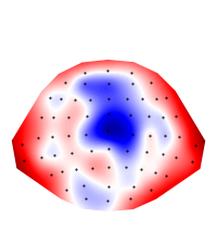
Out:

<Topomap: eeg>

Several methods allow aggregating data, for example an RMS over sensor:

eeg_rms = eeg.rms('sensor')
print(eeg_rms)
plot.UTSStat(eeg_rms)

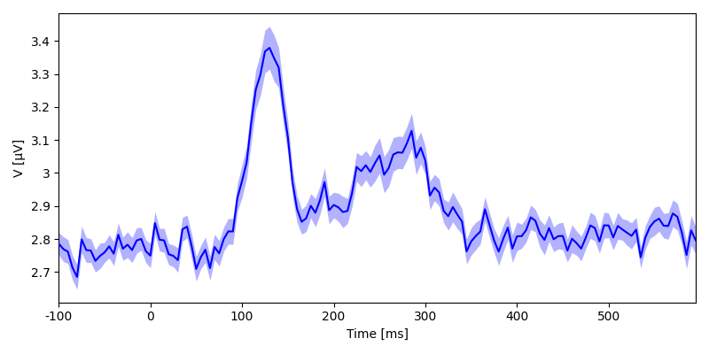
Out:

<NDVar 'eeg': 80 case, 140 time>

<UTSStat: eeg>

Or a mean in a time window:

eeg_400 = eeg.mean(time=(0.350, 0.450))
plot.Topomap(eeg_400)

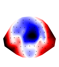
Out:

<Topomap: eeg>

As with a Var, the corresponding numpy.ndarray can always be accessed as array. The NDVar.get_data() method allows retrieving the data while being explicit about which axis represents which dimension:

array = eeg_400.get_data(('case', 'sensor'))
print(array.shape)

Out:

(80, 65)

NDVar objects can be constructed directly from an array and corresponding dimension objects, for example:

import numpy

frequency = Scalar('frequency', [1, 2, 3, 4])
time = UTS(0, 0.01, 50)
data = numpy.random.normal(0, 1, (4, 50))
ndvar = NDVar(data, (frequency, time))
print(ndvar)

Out:

<NDVar: 4 frequency, 50 time>

A case dimension can be added by including the bare Case class:

data = numpy.random.normal(0, 1, (10, 4, 50))
ndvar = NDVar(data, (Case, frequency, time))
print(ndvar)

Out:

<NDVar: 10 case, 4 frequency, 50 time>

Dataset¶

A Dataset is a container for multiple variables (Factor, Var and NDVar) that describe the same cases. It can be thought of as a data table with columns corresponding to different variables and rows to different cases. Variables can be assigned as to a dictionary:

ds = Dataset()
ds['x'] = Factor('aaabbb')
ds['y'] = Var([5, 4, 6, 2, 1, 3])
print(ds)

Out:

x   y
-----
a   5
a   4
a   6
b   2
b   1
b   3

A variable that’s equal in all cases can be assigned quickly:

ds[:, 'z'] = 0.

The string representation of a Dataset contains information on the variables stored in it:

# in an interactive shell this would be the output of just typing ``ds``
print(repr(ds))

Out:

<Dataset (6 cases) 'x':F, 'y':V, 'z':V>

n_cases=6 indicates that the Dataset contains 6 cases (rows). The subsequent dictionary-like representation shows the keys and the types of the corresponding values (F: Factor, V: Var, Vnd: NDVar).

A more extensive summary can be printed with the Dataset.summary() method:

print(ds.summary())

Out:

Key   Type     Values
-------------------------------
x     Factor   a:3, b:3
y     Var      1, 2, 3, 4, 5, 6
z     Var      0:6
-------------------------------
Dataset: 6 cases

Indexing a Dataset with strings returns the corresponding data-objects:

print(ds['x'])

Out:

Factor(['a', 'a', 'a', 'b', 'b', 'b'], name='x')

numpy.ndarray-like indexing on the Dataset can be used to access a subset of cases:

print(ds[2:])

Out:

x   y   z
---------
a   6   0
b   2   0
b   1   0
b   3   0

Row and column can be indexed simultaneously (in row, column order):

print(ds[2, 'x'])

Out:

Arry-based indexing also allows indexing based on the Dataset’s variables:

print(ds[ds['x'] == 'a'])

Out:

x   y   z
---------
a   5   0
a   4   0
a   6   0

Since the dataset acts as container for variable, there is a Dataset.eval() method for evaluatuing code strings in the namespace defined by the dataset, which means that dataset variables can be invoked with just their name:

print(ds.eval("x == 'a'"))

Out:

[ True  True  True False False False]

Many dataset methods allow using code strings as shortcuts for expressions involving dataset variables, for example indexing:

print(ds.sub("x == 'a'"))

Out:

x   y   z
---------
a   5   0
a   4   0
a   6   0

Example¶

Below is a simple example using data objects (for more, see the Examples):

y = numpy.empty(21)
y[:14] = numpy.random.normal(0, 1, 14)
y[14:] = numpy.random.normal(2, 1, 7)
ds = Dataset({
    'a': Factor('abc', 'A', repeat=7),
    'y': Var(y, 'Y'),
})
print(ds)

Out:

a   y
-------------
a   -0.19831
a   -0.068057
a   -1.2929
a   -0.2057
a   -0.030767
a   1.1981
a   0.85977
b   -0.24595
b   1.7527
b   -1.1674
b   -0.46498
b   0.089413
b   -0.43556
b   -0.032766
c   1.0152
c   1.178
c   1.8429
c   0.79221
c   3.601
c   1.2918
c   2.3041

print(table.frequencies('a', ds=ds))

Out:

a   n
-----
a   7
b   7
c   7

print(test.anova('y', 'a', ds=ds))

Out:

               SS   df     MS         F      p
----------------------------------------------
a           14.09    2   7.05   8.73**    .002
Residuals   14.53   18   0.81
----------------------------------------------
Total       28.62   20

print(test.pairwise('y', 'a', ds=ds, corr='Hochberg'))

Out:

Pairwise T-Tests (independent samples)

    b                  c
----------------------------------------
a   t(12) = 0.24       t(12) = -3.51**
    p = .815           p = .004
    p(c) = .815        p(c) = .009
b                      t(12) = -3.56**
                       p = .004
                       p(c) = .009
----------------------------------------
(* Corrected after Hochberg, 1988)

t = test.pairwise('y', 'a', ds=ds, corr='Hochberg')
print(t.get_tex())

Out:

\begin{center}
\begin{tabular}{lll}
\toprule
 & b & c \\
\midrule
a & $t_{12} = 0.24^{    \ \ \ \ }$ & $t_{12} = -3.51^{**  \ \ }$ \\
 & $p = .815$ & $p = .004$ \\
 & $p_{c} = .815$ & $p_{c} = .009$ \\
b &  & $t_{12} = -3.56^{**  \ \ }$ \\
 &  & $p = .004$ \\
 &  & $p_{c} = .009$ \\
\bottomrule
\end{tabular}
\end{center}

plot.Boxplot('y', 'a', ds=ds, title="My Boxplot", ylabel="value", corr='Hochberg')

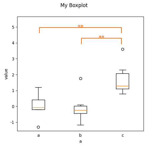
Out:

<Boxplot: My Boxplot>

Gallery generated by Sphinx-Gallery