Dataset basics

Load and prepare an example dataset:

# Author: Christian Brodbeck <christianbrodbeck@nyu.edu>
from eelbrain import *
import numpy
import pandas


df = pandas.read_csv('https://vincentarelbundock.github.io/Rdatasets/csv/psych/Tal_Or.csv')
data = Dataset.from_dataframe(df)
data['cond'] = data['cond'].as_factor({0: 'low', 1: 'high'})
data['gender'] = data['gender'].as_factor({1: 'male', 2: 'female'})

Inspecting datasets

The whole dataset can be displayed like any variable in iPython (in a plain text environment, use print(data)). For larger datasets it can be more convenient to print only the first few cases…

data.head()

#	rownames	cond	pmi	import_	reaction	gender	age
0	1	high	7	6	5.25	male	51
1	2	low	6	1	1.25	male	40
2	3	high	5.5	6	5	male	26
3	4	low	6.5	6	2.75	female	21
4	5	low	6	5	2.5	male	27
5	6	low	5.5	1	1.25	male	25
6	7	low	3.5	1	1.5	female	23
7	8	high	6	6	4.75	male	25
8	9	low	4.5	6	4.25	male	22
9	10	low	7	6	6.25	male	24

… or a summary of variables:

data.summary()

Key	Type	Values
rownames	Var	1 - 123
cond	Factor	low:65, high:58
pmi	Var	1 - 7
import_	Var	1:11, 2:13, 3:16, 4:26, 5:24, 6:23, 7:10
reaction	Var	1 - 7
gender	Factor	male:43, female:80
age	Var	18 - 61

Dataset: 123 cases

Individual rows and columns can be retrieved with common indexing:

data[10:15]

#	rownames	cond	pmi	import_	reaction	gender	age
0	11	high	1	3	1.25	female	22
1	12	low	6	3	2.75	female	21
2	13	high	5	4	3.75	female	23
3	14	low	7	7	5	female	21
4	15	high	7	1	4	female	22

data[2]

{'rownames': 3, 'cond': 'high', 'pmi': 5.5, 'import_': 6, 'reaction': 5.0, 'gender': 'male', 'age': 26.0}

data['age']

Var([51, 40, 26, 21, 27, 25, 23, 25, 22, 24, 22, 21, 23, 21, 22, 23, 23, 23, 22, 23, 22, 19.5, 61, 25, 23, 60, 22, 23, 22, 23, 25, 22, 23, 22, 25, 24, 24, 29, 24, 18, 23, 21, 24, 26, 24, 22, 21, 26, 24, 27, 26, 24, 24, 26, 24, 22, 23, 24, 24, 25, 23, 23, 23, 24, 18, 23, 25, 24, 23, 23, 24, 22, 24, 25, 22, 22, 23, 25, 23, 23, 24, 21, 23, 21, 23, 19, 25, 23, 22, 19, 23, 24, 32, 27, 25, 24, 23, 28, 24, 24, ... (N=123)], name='age')

Using datasets in functions

Datasets collect information describing the same cases (rows) on different variables (columns). This can simplify calling functions that combine information from multiple columns. Columns can be supplied as strings, and the dataset in the data parameter:

table.frequencies('cond', 'gender', data=data)

#	gender	low	high
0	male	19	24
1	female	46	34

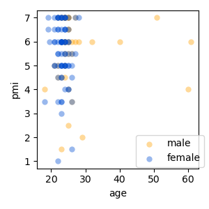
p = plot.Scatter('pmi', 'age', 'gender', data=data, w=3, legend=(.65, .2), alpha=.4)

These strings cannot only be keys, but they can be Python code that can be evaluated in the dataset. For example, if this is possible:

data.eval('age < 40')  # equivalent to `data['age'] < 40`

array([False, False,  True,  True,  True,  True,  True,  True,  True,
        True,  True,  True,  True,  True,  True,  True,  True,  True,
        True,  True,  True,  True, False,  True,  True, False,  True,
        True,  True,  True,  True,  True,  True,  True,  True,  True,
        True,  True,  True,  True,  True,  True,  True,  True,  True,
        True,  True,  True,  True,  True,  True,  True,  True,  True,
        True,  True,  True,  True,  True,  True,  True,  True,  True,
        True,  True,  True,  True,  True,  True,  True,  True,  True,
        True,  True,  True,  True,  True,  True,  True,  True,  True,
        True,  True,  True,  True,  True,  True,  True,  True,  True,
        True,  True,  True,  True,  True,  True,  True,  True,  True,
        True,  True,  True,  True,  True,  True,  True,  True,  True,
        True,  True,  True,  True,  True,  True,  True,  True,  True,
        True,  True,  True,  True,  True,  True])

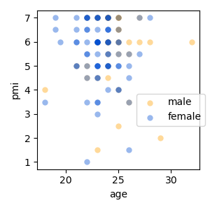
Then, this can be used directly for plotting:

p = plot.Scatter('pmi', 'age', 'gender', sub="age < 40", data=data, w=3, legend=(.65, .4), alpha=.4)

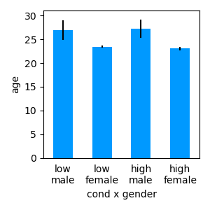
As in other cases, % is used to specify interaction between categorial variables:

p = plot.Barplot('age', 'cond % gender', data=data, w=3)

And * expands to main effects plus interaction:

test.ANOVA('age', 'cond * gender', data=data)

	SS	df	MS	F	p
cond	0.97	1	0.97	0.03	.860
gender	414.69	1	414.69	13.39***	< .001
cond x gender	3.02	1	3.02	0.10	.755
Residuals	3685.10	119	30.97
Total	4105.42	122

Constructing datasets

While datasets can be imported from external data sources, it is also often convenient to store new data in a table on the fly.

A dataset can be constructed column by column, by adding one variable after another:

# initialize an empty Dataset:
ds = Dataset()
# numeric values are added as Var object:
ds['y'] = Var(numpy.random.normal(0, 1, 6))
# categorical data as represented in Factors:
ds['a'] = Factor(['a', 'b', 'c'], repeat=2)
# A variable that's equal in all cases can be assigned quickly:
ds[:, 'z'] = 0.
# check the result:
ds

#	y	a	z
0	1.278	a	0
1	1.4323	a	0
2	0.35583	b	0
3	0.57962	b	0
4	-1.5772	c	0
5	-0.17162	c	0

An alternative way of constructing a dataset is case by case (i.e., row by row):

rows = []
for i in range(6):
    subject = f'S{i}'
    y = numpy.random.normal(0, 1)
    a = 'abc'[i % 3]
    rows.append([subject, y, a])
ds = Dataset.from_caselist(['subject', 'y', 'a'], rows, random='subject')
ds

#	subject	y	a
0	S0	-1.9398	a
1	S1	-0.075872	b
2	S2	0.84564	c
3	S3	0.77702	a
4	S4	0.46316	b
5	S5	-0.18091	c